Simon Lacoste-Julien
School of Computer Science, McGill University
Montréal, Québec, Canada
August 30, 2002
Abstract
This paper gives a detailed overview of the researches I did this
summer as a NSERC student with Hans Vangheluwe about Hybrid
Systems modelling and simulation, in the Modelling, Simulation and
Design Lab (MSDL) of McGill University. Hybrid Systems are
physical systems which are modelled with continuous components
(Differential Equations) as well as discrete components.
The three main parts of my researches this summer were to
get familiar with Hybrid Systems and implement some simple physical
models with the 522 Simulator1;
extend the 522 Simulator with a DAE solver written in Fortran
(DASSL and DASRT);
add a graphical interface for the modelling environment
using AToM3
I will describe each of those steps in this paper, as well as other related
tasks (like how to debug a shared library) which are worth being
documented with this project.
Why studying the modelling and simulation of Hybrid Systems? Well,
one reason was that this would involve mathematics, physics and
computer science, the three fields I'm majoring in; so this would
be interesting for me. But as important was that Hybrid Systems
are useful to model a lot of different physical systems: in
Chemistry for waste management systems; in Biology for feedback
control systems; in Mechanical Engineering for hydromechanical
systems controlling the direction of an aircraft (say); etc. The
ability to model those complex physical systems and to test them
(using simulation) can be greatly enhanced with a proper modelling
and simulation environment. So this explains why the development
of modelling tools like the 522 Simulator, as well as even more
general meta-modelling tools like AToM3 [which will be
explained in section 4], is useful. For an
introduction on Hybrid Systems, I refer the reader to a talk I've
given in the MSDL this summer:
MSDL Talk: Intro to Hybrid Systems Modelling [2].
It will be assumed in this paper that the reader is familiar with
Hybrid Systems.
The goal for me this summer was to get a feel for
multidisciplinary research and to get in touch with some of the
many issues about Hybrids Systems. The approach was originally on
the theoretical side, studying which could be the best formalism
to model Hybrid Systems and which could be the best formalism to
simulate them efficiently. But gradually, we went back to a more
pragmatic view and the researches were oriented in improving the
522 Simulator. This gave impressive results, and at the same time
gave us more insights about the theoretical sides of Hybrid
Systems [as will be explained in section 4.5].
I can separate my summer work mainly in three parts. The first
part was to read the literature about Hybrid Systems, to study the
522 Simulator and also implement some physical models with it in
order to find its strengths and weaknesses. This part is described
in section 2. One of the conclusions of this
part was that the modelling of complex physical systems would be a
lot simplified by the support of Differential Algebraic Equations
(DAEs) for the specifications of the system. So this motivated
the second part of my summer work, which was the extension of the
522 Simulator with a standard DAE solver, DASSL2 written by
Linda R. Petzold
and available on netlib. I didn't find
any Python version of DASSL, so I had to do the extension manually.
The fact that DASSL was written in Fortran made the task even more
challenging (and interesting). During this part, I learnt a great deal
of low-level stuff, but also useful stuff for a physicist who wants to
use older libraries written in Fortran; or for a computer scientist who
wants to glue applications together... Finally, the third
step was to build a graphical user interface for the modelling environment
of the 522 Simulator, using AToM3. With this tool, it is now
easier to ponder about ways to improve the modelling of Hybrid Systems,
as will be described in section 4.
I again refer the reader to
the talk [2]
the talk I have given this summer about Hybrid Systems. I will
give here a summary of the important points to remember.
The defining characteristic of a Hybrid System is to have discrete components as
well as continuous components. A finite state automaton (FSA) can model the
discrete transitions of the system, and a system of Ordinary Differential Equations
(ODE) can be put in each state to represent the continuous part of the system when
in this state (or 'Mode' of behaviour, as we'll see in a more formal description
of Hybrid Systems in section 4.2.1). The transitions between
different states (modes) are triggered by monitoring functions (also called
zero-crossing functions), which are functions of the state variables of the
system which trigger the transition when they reach zero. This forms a convenient
way to model 'state guards' on the mode. As a canonical example, we give in
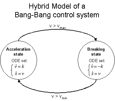
figure 1 the Hybrid Systems model of a bang-bang control system
of the speed of a car.
Figure 1: Hybrid model of a Bang-Bang control system using
FSA of ODE's. x is the state variable for the position of the car.
vmax and vmin are parameters which give the desired speed
range of the car.
The goal of this control system is to keep the speed of the
car between vmax and vmin. You can see the FSA structure as well as the
ODEs present in each state. The guards (like 'v > vmax') can be implemented
easily with a monitoring function like 'vmax - v' which triggers a transition
when it passes from positive to negative values.
This simulator was developed by Olivier Dubois and Eric McSween for the course
308-522A in Fall 2001 at McGill University (see
the web page describing their project, with the source code).
The name '522 Simulator'
was given by Hans and me when we were working with it during this summer.
The simulator is written entirely in Python. The modelling environment is textual:
you need to write a Python source file describing the model. This model can then
be loaded in a graphical simulation environment, where you can make multiple plots
of different state variables (either in function of time or in function of other
variables [phase plot]). The parameters of the model can also be changed from there.
The way the interfacing is done between a user model and the 522 Simulator is by
creating classes with specific content, which should inherit from standard
classes provided with the simulator. The required content of those classes
is described briefly in section 4.3.1. For screenshots and
examples of the 522 Simulator, see
my talk.
The 522 Simulator already supported any kind of ODE, with three different ODE solvers:
Euler, RK4 and an adaptive step size solver. It also supported the Discrete Event
Scheduling Formalism (DEVS), which means that you could define event handlers in
your model and schedule them in the future. For example, you can model a train
with passenger arrival events at random time (an example of such a model will
be given in figure 7, when the visual modelling
formalism I have built will be presented).
On the other hand, a feature that seemed to lack in the 522 Simulator was the
possibility to model the continuous behaviour of the system using Differential
Algebraic Equations (DAEs) instead of only ODEs. Indeed, most laws in Physics
are already expressed in a DAE format (like conservation of energy for two
point masses, for example:
m1 (d[r\vec]1/dt)2/2 + m2 (d[r\vec]2/dt)2/2 = E = const.).
It is often painful to transform those equations to explicit ODEs (and
sometimes impossible), so it would be nice if the simulator could do the job
at the place of the modeller. And this would permit the human modeller to focus
more on physical concepts rather than on the algebraic solving of the
equations. For those reasons, we have decided to include a DAE solver
in the 522 Simulator, step which will be described in the section.
DASSL is a standard DAE solver written by
Linda R. Petzold in Fortran in the 1980s and which has already been
used and tested extensively by the scientific community. The code
(ddassl.f3) is
available on netlib, but it needs some
intermediate routines (all available on netlib) which are not necessarily
easy to gather. A complete package is available
here, at a page
maintained by Laura R. Petzold. As mentioned before, I didn't find any
python version of DASSL on the web. DASSL was already included in the
Scilab distribution (a package
of scientific C and Fortran libraries in a user friendly environment),
but this wasn't in Python. Also, DASSL seems to have been included in
the scientific tool in Python SciPy, but
I didn't find any interface to use DASSL from Python in this distribution.
The solver we wanted to include in the 522 Simulator was DASRT,
a modified version of DASSL, which also supported the
monitoring function formalism. In other words, we could provide
DASRT with a DAE as well as a vector of zero-crossing functions
and it would detect if any zero-crossing functions had a zero during
a given interval; and find the zero if there was one. Since it took
a while before I succeeded to find the source file
ddasrt.f for the solver
on the internet, all the first tests for this project were done with
DASSL [but they have almost the same interface, so this was no big
deal].
I now give an overview of what was needed in order to extend the
522 Simulator with DASSL/DASRT. First of all, we wanted all
the user modelling to be done in Python, so this meant that
the DAE was a python function. This python function could be
passed to DASSL in order to be solved. DASSL was written in Fortran,
so this meant that I needed to find a way to call a Fortran routine (DASSL) from
Python and also that this Fortran routine had the possibility
to call-back a Python function (the DAE). Since Python provides
an interface with C only and not Fortran, a C wrapper needed to be build
between Fortran and C. This whole project of extension with
call-back mechanism has been separated in 5 steps, which are all
documented in the next subsections:
Learning the basics of extension in Python with a
call-back mechanism and test this with a simple Euler
solver.
Learning how to mix C and Fortran in a program.
Link step 1 and 2 by implementing a Euler solver in
Fortran and using it from Python.
Now that I have the basic principles to be able to
extend Python with DASSL manually, try to do it
automatically with f2py [with the Euler solver
first].
Finally, use all this knowledge to bring DASSL and
DASRT in Python.
3.1 Extending Python with C with call-back mechanism
A good reference to learn how to extend Python with C modules is
from the Python online documentation:
Extending and Embedding the Python Interpreter; or from
chapters 19 and 20 of Mark Lutz book: Programming Python
[3]. I present here a summary of the basic concepts
for the extension of Python.
First of all, let's clear out the vocabulary: extending
Python with a C module means to call and use a C program from
Python, which is the main program.
On the other hand, embedding Python in a C
module means to use Python from a C program, which is now the
main program. The first use (extension) is easier and is now easily
automated using SWIG (Simplified Wrapper
Interface Generator). The other use (embedding) is harder and there
is yet no standard tool to automate the process. This is due mainly to the fact
that there lacks a conventional way of doing
embedding, because C is a lot less ``standardized"
language than Python. Finally, extending Python with C with a call-back
mechanism means that Python will use a C program which can ``call-back" a Python
function. This is the method we needed in our project. It is thus some kind of
mixing of extension of Python (Python calls C)
with embedding (C calls Python). But one important difference with
embedding is that since Python is still the main program in this case,
there is no need to start a new Python interpreter as is needed
in the pure embedding case.
In order to have C code communicate with Python, you have to build
a C wrapper interface which will make the proper translation
of Python data to C data and vice versa. This wrapper uses the Python C API
to access all the standard functions of the Python interpreter, as well
as translation functions.
Those functions are made accessible in C by adding #include "Python.h"
in the C wrapper code. The other essential elements that need to be present
in the C wrapper code for a Python extension are the following:
Wrapper functions
You need one wrapper function per function that can
be called directly from Python. This wrapper function takes care of
translating Python arguments into C pointers; then calling the appropriate
C functions which execute what the function is supposed to do; then finally
another translation of the C returned value to a Python return value.
Registration table
This is a C struct that will give the association
between the names of the methods called from Python and their appropriate
C wrapper function that handles the method definition.
Initialization function
This is the function which is called by
Python the first time the C module is imported in Python. It takes care
of all the proper initialization. This is the only function which is
directly called from Python so it is the only one which should need external
linkage. The other wrapper functions should thus be declared static
for better encapsulation.
All those elements are present in the Euler example which will be presented
in section 3.1.4.
There are only two more elements which are needed in the C wrapper to also
implement the call-back mechanism:
Call-back pointer
This is a global variable of type Py_Object
which will hold the address of the Python function passed by Python
as an argument when calling some C function which needs a call-back.
The C wrapper of this function will initialize the value of the
call-back pointer when parsing the arguments given by Python.
Call-back wrapper function
This will be the function called by the C
code when wanting to call the Python function. It will first translate the
C arguments into Python arguments. Then it will call the Python function
(using the call-back pointer) using the PyEval_CallObject C/API function
which will return the result of the Python object as a Py_Object
pointer. Finally, the wrapper function will translate back this result into
C types and return this to the caller. So in brief, it does exactly
the opposite of what the normal wrapper functions do...
Unfortunately, those two elements are not present in the Euler example
I'll present in section 3.1.4 since all the C code was directly
included in the C wrapper, i.e., I wasn't calling any external C code, thus
I didn't have to build a call-back interface. On the other hand, the example
presented in section 3.3 which implements the Euler solver in Fortran
did show all those elements since in this case I was really calling external code
from my C wrapper [so the C wrapper was truly an interface; whereas in my
first example, the C wrapper was acting as both the interface and the
executing code].
As a first test in my extension project, I have implemented a Euler solver in
C that I wanted to use from Python. This solver would provide a single function
step(f,x,t,dt) where f would be a Python function representing the ODE
(a vector of functions gi(x,t) which returns the value of the derivative of xi
in function of x and t), x would be the state vector at time t; and this
step function would return an approximation of the solution vector x at time
t + dt using Euler algorithm [which is simply xnew = x + dt * f(x,t)].
The source file is given in appendix B.1 or can be found
here .
The Euler algorithm as well as the C wrapper are both contained in this file.
We'll describe how to compile it in the next section.
3.1.5 Compiling the extension module as a shared library
There are two ways to compile an extension module for Python: either statically,
or as a shared library. The static compilation means that you will recompile the
whole Python interpreter at the same time you compile the extension module and that
you will link everything together, statically. This method makes sense if you want to
provide additional functionality to the basic Python interpreter, or if your OS
doesn't support dynamic linking (using shared libraries).
In this project, we use dynamic linking since it is a lot more flexible (I can compile
different versions of the same extension module and test them one after the other
without having to recompile the whole Python interpreter) and thus faster to
develop. The basic principle of a shared library is that it postpones the
symbol linkage step to when the library will be imported into a running program
(the Python interpreter here), by storing the required information in the
shared object file.
The building of a shared library is quite system dependant. The best way to do
it portably for Python extensions is to use the Python tool Distutils
and to make a setup.py script. But before explaining this tool, I
will give an example of how to build Euler.c on Unix and Windows,
just as a reference.
Unix
For a Python extension on Unix, you need to build a shared object file
(.so). To do this, you would first do: gcc -c -fPIC -I/usr/include/python2.2 Euler.c -o Euler.o
where the -fPIC option is to produce Position Independent Code, and
the path appended to the include path option -I is the path to
the Python include directory which contains the Python header files
(Python.h, and others). You would then do the final linking
(here, there is none since I use a single file) with: gcc -shared Euler.o -o Euler.so
where the important option here is -shared to indicate that
we produce shared object code on Unix. Of course, we could have combined
those two steps here since we were only using one file. More information
about shared libraries on Linux can be found
here.
Windows
On Windows, we build a special kind of a Dynamic Link Library (DLL) which
has extension .pyd for Python. I give here what has worked on
my Windows XP machine with the MinGW
GNU compiler, but the safest way would be to use Distutils... I used
the MinGW compiler distribution since it also had the g77 Fortran
compiler and was one of the few Windows compilers supported by Distutils.
More information about DLLs can be found
here.
The building steps are the following. First, we build the object file
(almost the same as Unix): gcc -c -IC:\Python22\include Euler.c -o Euler.o
Then, we build the export list: a list of functions which
will be accessible from the importing program. In our case, we only need
to export initEuler. We put the list in a .def file,
with the following simple format:
LIBRARY Euler.pyd
EXPORTS
initEuler
This text is put in Euler.def. The final linking and building
of the shared library is then: gcc -mdll -static -s Euler.o Euler.def -LC:\Python22\libs -lpython22 -o Euler.pyd
where I needed to add the path to the Python library (the -L
and -l options) on my system.
Distutils
And now to do all this in a portable way, we write a setup.py
script which uses the module disutils. This is the
Python equivalent of a Unix Makefile. The minimal and simple
setup.py file I have used in this test is given in
appendix B.2 or can be found
here .
More information about how to build a setup.py file
for an extension module can be found in
section 3.3 of the online Python documentation
Distributing Python Modules. To use the
setup.py script, you simply type: python setup.py build
On Windows, you will need to add -compiler=mingw32
at the end of the command in order to specify which compiler
you want distutils to use. All the options and
library paths will be automatically given by distutils.
That's why this tool is portable. The shared library will
be automatically produced in a folder build/lib<platorm-name>/.
Finally, to use the shared library in Python, you simply need to
import it as a normal module. For the Euler example, we could do: >>> import Euler >>> Euler.step(f,x,t,dt)
assuming f, x, t and dt were
already properly defined. Appendix B.3 gives
the source file for test.py (also available
here ), a simple test for
my Euler solver extension. To use it, you simply
execute the function test.run().
Using the GNU compilers, it is possible to link C and Fortran object
files together. There are some compiler dependant issues to take
in consideration, though. The main one is name mangling. The
compiler sometimes changes the name of the functions when
compiling it to an object file, and this is done differently by
g77 and gcc. This means that in order to call
a Fortran routine from C (or vice-versa), the transformed name
needs to be known. A pragmatic way to do this is to try to link
the two objects file together, and then deduce what is the
mangled name by looking at the error message that the linker
gives. I will give a simple example of this below. A good
introduction to mixing C and Fortran is given
here.
A site from NERSC also provides some information on the subject
here.
As an example, I had created a program in Fortran which called
C; and another one in C which called Fortran. For both cases,
I was using the MinGW compiler on Windows XP (but the
same commands and files also worked on Linux). Let's consider the
first case.
The Fortran program (file fCallsC.f) was the following:
         PROGRAM fCallsC
            EXTERNAL HELLO
            CALL HELLO()
         END PROGRAM fCallsC
The simple C function which was called (file fhello.c)
was the following:
void hello_() {
    printf("Hello world! I'm in C!!");
}
The building commands were simply: gcc -c fhello.c g77 fCallsC.f fhello.o -o fCallsC.exe
The first command simply builds the object file of a C function
normally, whereas the second command builds the object file
of the Fortran program and do the final linkage of both object
files as well. First of all, note the underscore appended
to the name of the hello function in the C code.
This is the name mangling I have made reference to earlier. The
way I have found out how I should modify the name in C was simply
by trying to link both object files with g77, then
I received the error message: C:\DOCUME~1\Simon\LOCALS~1\Temp\ccM3aaaa.o(.text+0x7):fCallsC.f: undefined reference to `hello_'
So I deduced that the g77 had mangled 'HELLO' to
'hello_'. Also, I have to mention that you may have to
add some libraries for the final linkage step. In my case, using
g77 for the final linkage of the C and Fortran object
files worked without adding any library because by default g77
knew where to find both the C libraries and Fortran standard libraries. Note that
on my g77 installation, I could even compile both .c and .f files
with g77. On the other
hand, if I tried to use gcc to do the final linkage, I needed
to add the Fortran support library -lg2c.
Apart the name mangling issue, there are two other
important differences between C and Fortran that we need to take into
consideration when trying to mix the two.
Arguments passing
Arguments in Fortran are all passed by
reference; arguments in C are all passed by value.
This means that the C code should be modified accordingly
to use the right signature to call a Fortran routine (or changes
accordingly its signature in order to be called from Fortran).
All non-pointers types should send their address (using the ampersand
&) instead of their value. This will be shown clearly in
an example I've built in section 3.3.
Multidimensional arrays
Arrays indexing start at 0 in C, but
at 1 (or bigger if the user has required it) in Fortran. Also,
multidimensional arrays in C are stored in row-major order (row by row);
whereas they are stored in column-major order in Fortran. This means
that the value A[i][j] in C is the same as A(j,i)
in Fortran for an array A in memory. So basically, to solve
this issue, you simply inverse the indices in Fortran or in C.
An interesting tool is the header file
cfortran.h written
by Burkhard D. Burow and which provides a portable macro interface
between C and Fortran. This prevents us to have to worry about
the name mangling compiler dependant issue and other cross-languages
issues. A more detailed documentation for this tool can be found
here, written by Peter Daly.
Now that I knew how to extend Python with a C module with call-back, and that
I also knew how to call Fortran routines from C, I could combine
both mechanisms in order to extend Python with a Euler solver written in C.
I have modified the C wrapper built in section 3.1.4 so that
it wouldn't only act as an interface between C and Python, but also as
an interface between Fortran and C. The only elements that I needed
to add from the ones specified in section 3.1 were the
name mangling issue and the arguments passed by reference issue.
The Fortran code for the Euler solver is given in appendix C.1 or
is available here .
I have modified the interface of the solver in order to simplify
the wrapping. Instead of giving an array of functions to the solver
to represent the ODE, I gave it a function which would have the index
of the array as an argument. This permitted us to avoid to work
with array of functions in the wrapper. But it is good to mention
that the Fortran program wasn't changed at all to be interfaced with C.
It could have been used without changes from Fortran as well. All the
interfacing was done in the C wrapper. The code for the C wrapper
is given in appendix C.2 or is available
here .
You can notice in this code the presence of the call-back pointer and
the call-back wrapper, two elements not present in the Euler.c
file since I wasn't doing interfacing with an external file at that time.
Also, you can see how the Fortran routine was called: euler_(&length, callBack, x_array, &t, &dt, workArray);
Note the added underscore and the presence of the ampersands for the
non-pointer types so that to solve the name mangling issue and
the pass by reference issue. length was the number of equations;
callback was a pointer to the Python ODE function;
x_array was a pointer to the state variable array; t and
dt are explicit; workArray was a pointer to an array
which will hold the answer. This is also an important point to mention
since this is the usual way that a Fortran routine returns a value: by
changing in-place the content of a passed in variable. This will be
an important issue to consider when trying to use the DASSL routine
from Python. For example, to obtain the scalar result from a Fortran
routine, we'll have to create a 1 by 1 array in Python since
scalars are immutable in Python.
The building of a Fortran extension module is very similar to the
one in C except that we should use g77 in the final
linking stage. On the other hand, in order to build it in a
portable way using distutils, we need to use some
tricks since distutils doesn't support the compilation
of Fortran files.
In order to bypass this limitation, we compile the required
Fortran file as a library that will be included by distutils.
The code for this setup_fEuler.py file is given in
appendix C.3 or is available
here . The
main difference with the setup file for the Euler solver
in C is that this one uses library inclusion. So to build
the Fortran extension in a portable way here, we do the following:
We compile the Fortran solver: g77 -c Euler.f
We create a library for this object file: ar -cur libEuler.a Euler.o
We finally build the extension with distutils: python setup_fEuler.py build [--compiler=mingw32]
A simple test for this extension is provided in appendix C.4
or is available here .
It is used again by executing the function test_fEuler.run().
3.4 Automatic building of C/Fortran extension for Python
Building manually a C or Fortran extension for Python is very instructive,
but can be long, error-prone and not portable. It can be long because
of all the data translation overhead that you need to add around the function
calls. It can be error-prone because you have to manage the Python memory
of the created Python objects manually (using the reference counter
management functions Py_INCREF and Py_DECREF), and it is
easy to forget to increment a counter somewhere; especially when you are
extending a library like DDASRT.f which takes 20 arguments... Finally, unless
that you use a header file like cfortran.h [see section 3.2.3],
there are chances that your C wrapper for your Fortran extension is not
portable because of the name mangling issue.
Fortunately, there exists automatic C wrapper interface generation tools.
To extend Python with a C module automatically,
you can use SWIG,
as mentioned in section 3.1.1. This tool also supports the
handling of call-back functions as is explained in
this section
of the online documentation. But the interface to handle
call-back mechanism is quite low-level (and we even need to handle some
memory manually). On the other hand, the interface used by
f2py, a Fortran to Python
interface generator written by
Pearu Peterson,
is a lot cleaner. And this tool can even be used
(with some tricks) to extend Python with C modules [see
this email in the f2py discussion list for more info].
F2py
is a Python program which can generate automatically the C wrapper
extension file in order to extend Python with Fortran 77/90/95 routines.
This very useful tool is currently being developed
by Pearu Peterson. It provides
a efficient call-back mechanism, and can
also build automatically the extension module (compile and link
as a shared library) in
a portable way. With some hacks, it can also be used to extend
Python with C modules.
F2py works by using a signature file [.pyf] written in a
format similar to Fortran 90 and which describes the signatures
of the functions which should be available from Python. F2py can
generate automatically this signature file by reading the Fortran
source code, and the user can modify it for the fine-tuning of
the specifications. Unfortunately, the user guide currently
[August 30, 2002] available on the f2py web site is quite outdated4.
But Pearu Peterson is currently working on a new version of the
documentation, which is available here. We'll describe in the next section how to use f2py
to extend Python with our Euler.f example. But before,
here are several notes to take in consideration:
I was using version 2.13.175-1250 of f2py.
On Windows, I was using the mingw gcc compilers, which
works nicely with f2py. Depending of which version
of f2py you use, it could happen that you need a patch
to make it works with mingw. See the end of
this email for the
patch.
3.4.2 Using f2py to extend Python with Euler in Fortran
The usual way of using f2py is to first produce a signature
file with, for example: f2py -h f2pyEuler.pyf -m f2pyEuler f2pyEuler.f
The -h option gives the name of the signature file generated;
the -m option gives the name of the extension module created
and f2pyEuler.f is the source file to be scanned.
And then (after modifications of f2pyEuler.pyf if necessary),
we can build the shared library for the extension module with: f2py -c f2pyEuler.pyf f2pyEuler.f
The -c option is to tell f2py to build the extension module.
If any .pyf file is included, it will use its specifications
for the signature. You need to put all the needed source files also
as arguments (here f2pyEuler.f).
F2py is quite intelligent to guess the signature of the functions,
and even of the call-back functions if those were called explicitly in
the source file.
But in the case of arguments which will be changed in-place (like in most
of old Fortran 77 code), the user has to manually indicate the intent(inout)
of those variables in the signature file. The main attributes used by f2py
in the signature file are well-explained in the
old user guide.
The intent(<intentspec>)
attribute specifies how a variable is going to be used in a routine. The main
ones needed for basic uses are: intent(in) which means that the
variable is an input variable and is assumed not to be changed by the function;
intent(out) which means that the variable is only an output variable
(f2py will then generate a different Python signature than the Fortran one
for this function, see the
old user guide for more details); and
intent(inout) which means that the variable is used as input AND output,
and can be changed in place by the Fortran routine (or the Python one when in the
specification of a call-back function). When there are only a few modifications needed
for the signature file, those can be directly included in the Fortran source file
using the cf2py tag at the beginning of each line. In the case
of our Fortran Euler solver (which was already described in section 3.3),
we only needed to add the specification that two variables were used as arguments
which could be changed in-place; all the rest of the signature was correctly
detected by f2py. So the following two lines were simply added to the file
Euler.f (to yield the f2pyEuler.f file which is available
here ): cf2py intent(inout) res cf2py intent(inout) newx
With this modification, we could build directly the extension module from
the source file, without using the intermediate .pyf file: f2py -c f2pyEuler.f -m f2pyEuler
We still needed to specify the module name for the extension module (using
the -m option) since this wasn't specified in the source file.
This command will produce a f2pyEuler.so shared library which
can then be used as before. A test script for this extension is available
here . Note that the
numpy package was needed
since f2py uses only Numeric arrays.
Finally, after all these testing steps, we were ready to accomplish
the goal for this part of my summer research: extending Python with
the DAE solvers DASSL and DASRT.
The source files used for DASSL were downloaded from
here, at a page
maintained by its author,
Linda R. Petzold. This package contained ddassl.f, the main source file,
as well as daux.f and dlinpk.f which contained the auxiliary
linear algebra routines needed. All the documentation for the solver is given
in the source file. The first version of the signature file
(called dassl.pyf) was produced with: f2py -m ddassl -h ddassl.pyf ddassl.f only: ddassl
The only: ddassl option was to specify that only the ddassl
routine present in the source file was to be exported; the other routines
were ignored. Then, I have modified the ddassl.pyf file
to add the intent of each variable, as well as the definition
of the call-back routines. The new signature file is given in
appendix D, or is available
here .
The final compilation and linkage was done using f2py -c ddassl.pyf ddassl.f daux.f dlinpk.f
Note the presence of all the required source files, as well as the modified
signature file. This produced ddassl.so which can be tested
with a Python script available here
here .
The signature for Fortran is: DDASSL(RES, neq, t, Y, YDOT, tout, INFO, rtol, atol, idid, RWORK, lrw, IWORK, liw, RPAR, IPAR, JAC)
Here is a brief description of each argument (all this info can also
be found in its documentation):
RES
This is a subroutine provided by the user which
represents the DAE system to be solved. More info about its
format will be given in section 3.6, when I will
explain how to use DASRT from Python.
neq
An integer representing the number of equations of
the system.
t
The current value of the independent variable (time).
This variable is modified in-place by the solver as it solves
the equation (and time advances). This means that it should be declared
as intent(inout) in f2py.
Y, YDOT
These arrays contain the solution components at t
and its derivatives (respectively). They are also modified by the solver
as time advances (this is how the user can find back the solution at t).
tout
The time at which the solution is desired.
INFO
This is an integer array of size 15 which gives information on how the
solving task must be carried out. For a default use, all components should
be equal to 0.
rtol, atol
Those quantities represent the relative and absolute
error tolerance which are provided by the user. They can be modified
by the solver.
idid
This scalar communicates to the user what the solver did.
RWORK, IWORK
These are real and integer work arrays for the solver,
respectively of length lrw and liw.
RPAR, IPAR
These are real and integer parameter arrays respectively
which can be used by the user to communicate between the calling program and
the RES and JAC subroutines.
JAC
This is a subroutine which can be provided by the user to
compute the Jacobian matrix (of partial derivatives) of the DAE. If
INFO(5) is set to 0, then the Jacobian is computed
automatically by DASSL; if it is set to 1, then DASSL uses the
JAC subroutine provided instead.
I gave here only enough information so that the reader can understand roughly
how DASSL can be used, and also the subtleties of its extension. For a more
complete presentation, please consult the documentation in ddassl.f.
Several points are worth mentioning here. First of all, as was
mentioned by Pearu Peterson in
this email
on the f2py discussion list,
this compilation process can be made more convenient by using the
scipy_distutils tool. With this modified version of the
distutils module, you can specify Fortran files and .pyf
files in the source list for a setup.py script. This also
gives you a more convenient way of compiling Fortran extension modules
portably than building Fortran libraries as I had explained in
section 3.3.1. I haven't investigated how to use
scipy_distutils, though. It seems the information can be
found on the SciPy website.
Secondly, because f2py is still in development process, it
could happen that there are bugs with your generated extension module.
To try to debug your extension module, you can use the -debug-capi
function while building it with f2py: this will make the C wrapper interface
to be very verbose about what it is doing. You can then post the bug to Pearu
Peterson on the
f2py discussion list; he
usually answers email very rapidly.
In my case, once I had figured how to do the extension properly, everything has
been working fine. But before I got there, I passed through a lot
of debugging and segmentation faults (the omnipresent bug when working with
extension modules)... I have explained how to debug shared
libraries using gdb in appendix A, because I think
it is very useful to understand
the working of extension module. This was the only
way in which I have succeeded to find the source of my segmentation faults.
These came from a subtle point, so it's worth mentioning here. Fortran supports
happily unbounded arrays (i.e. array without any bound declared), and those
were used heavily in ddassl.f. On the other hand, to translate
Fortran arrays into Python arrays, you need to specify the bounds. So that's
why that the bounds of any array used in a call-back function need to be
declared. This wasn't checked by the version of f2py I was using so it
produced happily an extension module which could crash. On the other
hand, you can use unbounded arrays in the signature of a routine
called by Python since Python keeps the size information with its arrays.
So that's why I could use unbounded arrays (using dimension(*))
in the signature of the ddassl routine given in
ddassl.pyf (see appendix D), but all the
arrays used in the call-back routines signature (RES and
JAC) had their bounds declared. In my test Euler solver in
Fortran (see section 3.3), I had passed the size of the state vector
(which corresponded to the number of equations in the ODE) as an argument
of the call-back routine. There was no such argument in the signature of the
call-back functions used in ddassl.f, so a trick was needed
in order to know what was the size of the arrays. The IPAR argument
in the call-back functions was an integer parameters array which could be
used by the user to communicate between the caller of DASSL and the call-back
routines. I used as a convention that the three first elements of IPAR
represented the dimensions of the needed arrays (see my modified ddassl.pyf
file).
In the case that you would want to study the C wrapper file generated by the f2py,
you can produce it by executing f2py without the -c option on the
.pyf file: f2py ddassl.pyf
This will produces the C wrapper file dasslmodule.c (since the module name
given in in ddassl.pyf was dassl).
If you want to reinstall a new version of f2py (this could happen if you're unlucky
enough to download a buggy version of f2py), you can simply delete the content of
<path to your python>/lib/site-packages/f2py2e, and then reinstall
the new version normally.
Finally, note that the interface I have built with DASSL is very primitive.
F2py provides very powerful features to modify the functions signature in a clean
way (for example, it could automatically provide the work arrays; it could
copy the input arrays that need to be modified in-place and return the copy [so
without disturbing the original arrays, as shall be expected in a Python
way of passing arguments]; etc.). With these changes, the way to call DASSL
from Python could be simplified a lot. But for two reasons, I have decided
to use the simplest way of interfacing DASSL with Python (simply recopying
the Fortran signature in Python). First, most of the f2py features which
could accomplish that were no more documented, so it was tricky to use
them. Secondly, I was not sure how I was going to use DASSL from Python
yet, and it would be easy to build a wrapper in Python around the imported
ddassl extension module in order to give a cleaner interface. Since I was
building only a prototype, the primitive interfacing was enough.
An example of question that could arise when trying to develop an efficient
implementation of the solver in Python could be: is copying the input array
automatically by f2py (as mentioned above) really a good thing? For example,
if we run DASSL in intermediate mode, the control could pass very often
between Python and ddassl.f, and each time f2py would do a copying
of the input array. On the other hand, doing the copying only once in
Python when starting the solver (and not each time the solver is
called) would avoid all this overhead. This kind of question
explains why I have postponed the clean interfacing of the solver
after the development of the prototype.
I have also to mention that using
intent(inout) arguments in my interface is against the philosophy
of Pearu Peterson, who suggested to use always intent(in, out)
instead. This issue is discussed in
this email. From what I have understood, using intent(in,out) has
two main effects: it will append the variable as a return value in a tuple for
the function; it will make the changes to the variable more robust than
if intent(inout) had been used (for example, it seems that when
intent(inout) is used, it could happen that changes to the variable
made by the Fortran code could not be transmitted to Python under
certain conditions). But because I wanted to mimic the Fortran interface in
Python for simplicity, I decided to still use intent(inout)
for the arguments of my interface function in DASSL.
DASRT has exactly the same signature as DASSL, but with three more arguments: DDASRT(RES, neq, ... , JAC, G, ng, JROOT) G is the subroutine for defining the zero-crossing functions
(G(t,Y)) whose roots are desired during the integration (so is
a call-back routine);
ng is the number of constraint functions (if set to 0, then DASRT
operates the same as DASSL); JROOT is an integer array of size
ng used to output the root information (JROOT(i) = 1 if
the ith zero-crossing function had a root during the integration).
How it can be used is explained in section 3.6. The building
of the DASRT extension to Python is very similar to DASSL. The only difference
is with the new three arguments, and the added call-back function G.
The signature file I have used for it can be found
here .
You can build it with: f2py -c ddasrt.pyf ddasrt.f daux.f dlinpk.f ddassl.f dlamch.f lsame.f
The source files and a
python test script can be obtained by clicking on their
respective link . I have to explain the origin of the source files
I've used, though. There is a bug in the [current version of the]
ddasrt.f program available
on netlib: namely, the derivative vector YDOT is not updated
when the integrator is stopped after having found a root in the
constraint functions. This bug was corrected in a version of DASRT which is
distributed in the Scilab source
files. So I have taken ddasrt.f from the routines/integ
directory of the source files of Scilab-2.6; dlmach.f and
lsame.f from the routines/lapack directory; and the remaining
linear algebra routines were taken from daux.f, dlinpk.f and
ddassl.f which were the same sources as used before to build DASSL.
This mixing of Scilab source files with the auxiliary routines used by DASSL was
the simplest way I have found to make DASRT works.
3.6 Inclusion of those solvers in the 522 Simulator
The best test for each of the extension modules built above was to
use them in a real simulation environment, so they were added in the 522 Simulator.
All I needed to do was to add a small layer of Python code to interface the new
solvers with the simulator: namely, I only had to build a solver class with
a step function with the correct signature. The file which contained
the code for the solvers
in the 522 Simulator was Solver.py; the modified version can be found
here
. Note that since the 522 Simulator doesn't support
yet DAEs at the modelling level, DASSL and DASRT were used as mere ODE solvers.
But by looking at the code of Solver.py, you can have a good idea
of how to use DASSL and DASRT from Python and what format should have
the RES, JAC and G functions. I have to mention
one important issue when trying to interface DASSL or DASRT with Python: all the
scalars which are used as input as well as output in DASSL (the time t)
for example, were declared as 1 by 1 Numeric array since scalars are immutable in
Python so cannot be changed in place as is required by the Fortran code.
The code for the 522 Simulator with the new solvers can be found
here . This comes with all the solvers
already built on Windows and Linux
(.pyd and .so). In case they don't work on your machine, you can rebuild all of
them by following the instructions given in the readme file in each
Solvers_build/ subfolder, and then move the rebuilt solvers in the
root directory (Simulator522/). Each subfolder also contains a little Python
test script to test the solver (the same that were given in this document). In order
to run the 522 Simulator with the new solvers, you will need numpy. And you will
of course need f2py if you want to rebuild some of the solvers. To start the simulator,
you simply execute the module GUI_new.py.
This part of my summer research has permitted me to explore useful tasks
in the world of modelling and simulation: extending Python with Fortran
code with call-back mechanism, and doing this automatically with
f2py. Now that the DAE solver has been added to the
522 Simulator, the next step will be to add the DAE support in the
modelling environment (since for now, we can still model only with
ODEs). Other improvements for the 522 Simulator will be suggested
in the conclusion of this report (section 5.2).
4 Building a GUI modelling environment for the 522 Simulator
The third step of my summer work was to build a graphical modelling
environment for the 522 Simulator. Adding a GUI modelling environment
for the 522 Simulator has several advantages:
A GUI is usually more user friendly than raw code and it permits
the user to focus on the model rather than how to implement it for
this particular Simulator.
To build a good GUI, you need precise specifications; so this
pushed us to really think about what we wanted to include in our
Hybrid Systems formalism. Those specifications (in the meta-model which
will be explained later) also permit model checking at the syntax level
(using constraints in AToM3).
By adding another layer of interface between the simulation
environment and the modelling level, we can obtain a yet cleaner interface.
For example, there was some repetition required in the Python code for the
models in the 522 Simulator (as for the variable initialization for example),
and you often needed to add self. at many places. In the GUI
I have made, you don't need all this redundancy (which was error prone and
time consuming): you only need the (almost) ``minimal" information
required to specify the model.
On the other hand, the disadvantage of a GUI is that you have less flexibility
than raw code, i.e. you only have access to the features that the designer
of the GUI has decided to provide; whereas you normally can do almost
anything when you code in Python. This is not as bad as it seems, since
there is always a compromise to do between flexibility/freedom, and
model checking/correctness.
The building of a GUI for the 522 Simulator was done in two steps: first of
all, the specifications for the modelling environment for Hybrid Systems
were given to AToM3 which could then generate automatically a
modelling environment tool (see section 4.1). Secondly,
I wrote a code generation tool (using graph grammars in AToM3) which
could transform a Hybrid Systems model instance built in my GUI to
a model instance understandable by the 522 Simulator (i.e. in Python code
with the original interface of the 522 Simulator).
Before explaining those two steps, I'll give a brief introduction
to Meta-Modelling with AToM3.
Before constructing models in a specific formalism (in our case,
the Hybrid Systems formalism), we need to specify the rules and meaning
of this formalism. This specification could also be considered as a model
in its own right. But since it is a model of a formalism, and a formalism
is viewed as a setting to build new models, we'll call the model of the
formalism a meta-model (i.e., a model for models). So when we specify
the rules that will regulate the building of a Hybrid Systems model, we are
truly specifying the meta-model. Usually, meta-models are defined in some
mathematical setting (set theory, logic, graph theory, etc.). But there
are some visual formalisms which can be well-suited to build them,
as for example the Entity-Relationship formalism (ER) [which can be described
briefly as entities connected by relationships]. Since we are building
meta-models in this formalism, we'll call it a meta-formalism, and the
specifications of ER are given in a meta-meta-model (in a model of
meta-models)5.
This being said, we can now present AToM3.
AToM3 stands for
``A Tool for Multi-formalism and Meta-Modelling''. It was developed originally by
Juan de Lara Jaramillo and
Hans Vangheluwe at the MSDL of
McGill University. AToM3 is a visual tool to write meta-models and generate
automatically the (code for the) modelling environment corresponding to the meta-model;
and also to write and execute formalism transformations (using graph grammars, since
(almost) everything in AToM3 is represented internally by graphs). A
good tutorial about meta-modelling with AToM3 was written by my
colleague Marc Provost. The
following paper [4] also gives a good introduction on how to
create modelling environment with AToM3. In this case, the example presented is
the building of a modelling environment for simple Causal Block Diagrams
(CBD) and the generation of code in the
Object-Oriented Continuous Simulation Language (OOCSMP)6. My approach in this project is thus very
similar: I write a meta-model for Hybrid Systems and a code generator
for the 522 Simulator language.
This section describes the building of the specifications for our
Hybrid Systems formalism. Basic knowledge of AToM3 will be assumed.
A visual formalism can be defined by
a syntax, a set of constraints and a set of visual appearances for its
entities. All this can be done easily with AToM3.
Its semantic can be given by mapping the formalism to another
formalism (in our case, we map our Hybrid Systems models to the 522
Simulator formalism), and this can be done using graph grammars transformation
with AToM3. This last part will be explained in
section 4.3, but the semantic of our Hybrid Systems
formalism will also be explained informally at the same time we describe our
meta-model here.
Figure 2 gives a screenshot of the meta-model for Hybrid Systems
(HS) that I've built with AToM3.
Figure 2: Meta-model of Hybrid Systems in AToM3
I will first give a high-level description of the meta-model.
The meta-model was directly inspired from the informal description of
Hybrid Systems that I had given in section 2.1.
It consists of a mix of FSA, ODE and DEVS.
The two entities in the meta-model are used
to model the hybrid behaviour of a HS: the Mode entity represents a possible
continuous mode for the system (e.g. free_fall, accelerating, braking, etc.) (and
so contains the ODE);
the Event_HS7
entity represents a possible discrete event which can happen (like
start_braking, start_accelerating, collision, etc.) (and so represent the
events in the DEVS). A Mode node
will contain a ODE describing the state of the system in this mode.
The monitoring functions used in this mode are represented by State_Guard
relationships connecting Mode to Event_HS, the latter identifying
which event is triggered when a zero has been detected in the given monitoring
function. The Event_HS node will contain action code which will
represent what is happening when the event is triggered. The event can also
schedule new events using a Schedule relationship; and can cause
a mode transition using the Mode_Transition relationship
(this represents the transition for the FSA).
The variables and parameters used in the model are entered as global model
attributes. The file used to save the meta-model was
HybridSystems_ER_mdl.py8. It can be found
in the HybridSystems folder which contains all the files
needed for the new 522 Simulator (a link to it will be given in
section 4.4). Note that for the remaining of this part, all the paths
will refer to subdirectories of the HybridSystems folder.
Note that with the modelling environment specified
by this meta-model, you can express a lot of different Hybrid Systems
models. You can use the event scheduling component to implement if-constructs
and while-loops, so this means that you can express almost any computable
function. I think that anything that could be added to the modelling environment
could be considered simply as `syntactic sugar' to facilitate the modelling
(like implementing a real while-loop construct).
From this meta-model, AToM3 generated automatically the code
for the modelling environment, in the file HybridSystems.py.
Some modifications were done manually to the modelling environment
using the Button formalism to add three buttons (explained later).
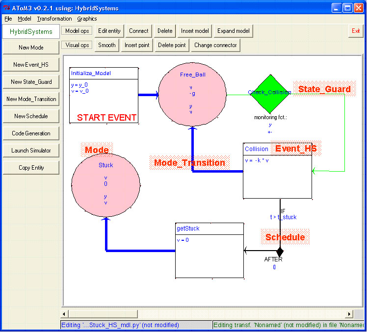
The obtained modelling environment is shown in
figure 3. You can see in the canvas an example
of a very simple model of the Hybrid Systems kind:
a bouncing ball
with the added property that it can get stuck after a certain amount
of time (this simple but weird property was used to demonstrate the
possibility of scheduling new events in the formalism). Five labels
in red were added manually in the figure to identify the graphical
appearance of each of the five types of entities9 that can be
drawn in the canvas: Mode, State_Guard, Event_HS, Schedule and
Mode_Transition. The buttons at the top of the modelling environment
(Edit entity, Connect, Delete, etc.) are the usual ones provided by
any modelling environment of AToM3. The five first buttons
on the left (New Mode, etc.) were automatically generated by
AToM3 (as usual) from the meta-model given in
HybridSystems_ER_mdl.py. The next three buttons were added
manually by modifying the generated code in HybridSystems.py
using the Button formalism. The Code Generation button launches
the graph grammar which will produce code understandable for the
522 Simulator, from the model (see section 4.3). The file
containing the code for this button is
code_for_codeGen/button_gen522Code.py. The Launch Simulator
button starts the 522 Simulator; its code is given in
code_for_codeGen/button_Start_Simulator.py. Finally,
the Copy Entity button can be used to copy entities built in the canvas;
it is particularly useful to copy a Mode which contains complex ODEs which
don't change much from one Mode to the other. Its code is given in
code_for_codeGen/button_copy.py. Note that this feature
will be included eventually directly in AToM3.
Figure 3: Model of a Bouncing Ball in the HS formalism
The labels in red identify the graphical appearance of the different
types of entities in the model.
Now, let's have a look at this example of Hybrid Systems model
(figure 3). What we wanted
to model was a bouncing ball, which can get eventually stuck on the ground
after a certain time (say, for example, that a trap appears in the ground after
a certain time). I have used two modes for this system: when the ball was in
free fall (Mode Free_Ball) and when it was stuck (Mode Stuck). When in free
fall, the ODE for the ball is simply dv/dt = -g and dy/dt = v where y is
obviously the height of the ball; v, its speed; and g the gravity constant.
(I will explain in section 4.2.4 what is the syntax to define ODEs).
When in the Stuck mode, the ball is simply at rest so that dv/dt = 0. The
first event in the model is the Initialize_Model event, which is labelled
as being the Start Event. In any HS model, there needs to be exactly one
Start Event which will indicate where to start the simulation. This event is
usually used to initialize the state variables in the model (here, the action
code in the event says ``y = y0; v = v0'' so the height and speed
of the system are obviously initialized to the value given by parameter y0
and v0 which are defined in a global attribute for the model (namely,
in Parameters_List). There is a Mode_Transition going from the start event
to the Free_Ball mode indicating which mode is used as the first mode for the
simulation. For correct simulation of the model, it is mandatory that the
Start Event be linked to a Mode. This is not checked automatically (yet)
by the modelling environment, but it has to be there. In case there is
nothing continuous happening at the beginning, you can simply link the Start Event
to a mode with an empty ODE (like was done in the Train example which will
be presented later (figure 7), in the Train_at_rest mode).
The Check_Collision State_Guard is connecting the Free_Ball Mode to
the Collision Event_HS, with the meaning that when a zero is detected
in the monitoring function given in the given State_Guard attributes
(here, y as is shown graphically) in the correct direction (here, from + to -),
then the given Event_HS is triggered, i.e. its action code, mode transition and
schedule events are executed. In this case, Collision contains only the line
v = - k * v as action code, which reverses the speed of the ball with a coefficient
of restitution k (will be smaller than 1 for inelastic collision; equal to 1 for
elastic collision; and greater to 1 for superelastic collision). The Mode Transition
to the Free_Ball mode indicates that after this (instantaneous) event, the system is
put back to the Free_Ball continuous mode. But there is also a Schedule relationship
which connects the Collision event to the getStuck event. The condition for the
scheduling to occur is shown graphically with IF t > t_stuck, i.e. the event
getStuck will be scheduled in 0 second (because of the AFTER 0) if t (time) is
greater than the parameter t_stuck. The event getStuck simply sets the speed to 0 and
then puts the system in the Stuck mode.
So an informal denotational semantic for this model in the (informal)
ODE + control flow formalism could be the following:
initial conditions:
y = y_0
v = v_0
initial ODE:
dy/dt = v
dv/dt = -g
when y = 0:
    if t > t_stuck then:
        v = 0
        use empty ODE for the remaining of the run (dy/dt = 0; dv/dt = 0)
    else:
        v = -k*v
Figure 4 shows the results of the simulation
of this model using the 522 Simulator (the model file used was the one
generated automatically with the Code Generation button).
Figure 4: Simulation of the Bouncing Ball model with the
522 Simulator. The solver used was RK4 with time step of 0.1. You
can see that after t = 80, the first collision yields
the ball stuck to the ground (as required).
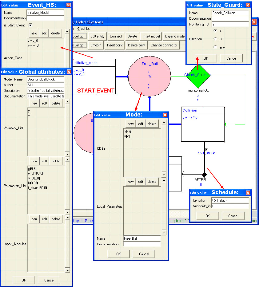
Figure 5 shows more details about the meta-model
for Hybrid Systems. All the attributes for each entity are shown, plus
the graphical appearance of the Mode and Event_HS entities. The cardinality
of each connection was also added in red. Here is a
description of each attribute for each entity (we refer also the
reader to consult figure 6 at the same time; the
latter gives the content of the attributes for the Bouncing Ball example):
Global attributes:
Model_Name
A string for the name of the model.
Author
The author(!).
Description
A short description for the model. It will
be included in the generated code.
Documentation
More documentation for the model (as what
each variable represents; where special care should be
taken with parameters, etc.). It will also be included
in the generated code.
Variables_List
A list of strings giving the names
of the variables used in the model.
Parameters_List
This is a list of tuples
(see figure 610
) of strings, to define
the global parameters used in the model. The first
element (string) of the tuple represents the parameter name;
the second string gives what is the initial value for the
parameter.
Import_Modules
This is a list of strings representing
Python modules that the user want to use in commands inside
the model. For example, the random module can
be used to produce random numbers (see the Train example,
section 4.2.5).
Mode attributes:
ODEs
A list of tuples of strings representing the ODE for
the continuous mode: (<variable on LHS of ODE>,
<allowed python expression for derivative>).
The first element of the tuple is the variable
name that is differentiated with respect to time (LHS of the equation);
the second element is a (Python) expression giving the RHS of the equation.
For example, dv/dt = -g is encoded with a tuple ("v","- g"). Notice the
space between the '-' and the 'g'; this is because ANY model variable name
or parameter name used in the expression needs to be separated by a
space for the correct parsing of the expression when generating code.
Only variable names already defined in the global attribute Variables_List
are allowed as the first element of the tuple. What is allowed in the
expression string in the second element of the tuple is any Python expression,
with the restriction that variable or parameter names
be separated by spaces. You can use external module functions <module_name>.<method>
provided that <module_name> was defined in the Import_Modules global attribute.
Also, to define non-autonomous ODE, you can simply use the special variable 't'
which represents time.
Local_Parameters
A list of tuples of strings representing
declaration of local parameters to the mode:
(<parameter_name>, <init_expression>). If the <parameter_name> is the
same as one already declared at the global level (in Parameters_List),
then it will override the latter. The <init_expression> is the initialization
expression of the local parameter, and have the same syntax and restriction as the
derivative expression in the attribute ODEs. But the meaning of a state variable
in this expression is the value of the variable when entering the
mode. For example, having (k,v) with v a state variable would mean that the
local parameter k is set to the value that v has when the system is
entering the mode. Similarly, 't' will mean the time when the system
is entering the mode. Finally, you may (for convenience) use other local
parameters in the expression of the RHS with the condition that you are careful
with the order in the list: you can only reference local parameters which were
defined before in the list. This can be useful if you want to build complex
expression with lots of constants in steps.
NOTE: there is no way the value of the local parameters can be changed from outside
the mode (for example, by an event). If you want to change parameters
with events, you have to define them as global parameters by putting them in the
Parameters_List global attribute.
Name
The name of the mode (must be unique).
Documentation
Documentation for the mode (will be added at the corresponding
place in the generated code).
Event_HS attributes:
Name
The name of event.
Documentation
Its documentation (will be put as a comment in the generated
code in the definition of the respective event handler).
is_Start_Event
This is a boolean to indicate if the given event
is the Start Event, i.e. the first event that will be executed when
simulating the model (you should have exactly one Start Event in the model;
this is usually where you also do all the state variable initialization).
The value of this boolean influences the appearance of the event in the model.
Action_Code
This is a list of strings which represents a list of actions
to execute when the event is triggered. Each string represent a line of a
Python statement. You can use again model variable names and global parameters if
they are separated by spaces. You can use 't' for time. You could even do loop
and stuff by formatting it properly (e.g.: build the list
("for x in [1,2,3]:", " print x") ).
TRICK: In order to make reference to a local parameter in the current mode
(i.e. the mode of the system WHEN the event is triggered), you can use the
special construct self.diffeqs.<param_name>.
State_Guard attributes:
Name
The name of monitoring function.
Documentation
Its documentation (will be put as a comment in the generated
code in the definition of the monitoring function).
Monitoring_fct
This is a string which represent a Python expression which
gives the return value of the monitoring function. The syntax and restriction
for the expression is the same as the one for the derivative expression
in the ODEs attribute in the Mode entity.
Direction
This is an enum in which you choose which direction of crossing
that will be monitored by this function ('+-' is from positive to negative;
'-+' is for the opposite; 'any' is for any direction).
Schedule attributes
Condition
This is a string representing a boolean expression in Python
(0 is false, non-zero is true). It can use model variables, parameters, time 't',
external module functions, etc. as in the ODEs attribute of the Mode entity
(except it can't make direct reference to local parameters).
Schedule_in
This is a string representing an arithmetic Python expression
which will tell in how long the connected event will be scheduled in. For the
syntax, it has the same possibilities as for Condition.
Mode_Transition attributes
It has none.
Figure 5: Details of the meta-model of HS.
Several dialog boxes from AToM3 are shown; the red arrows were added
for more clarity; the red numbers are the cardinality of each connection.
Figure 6: Examples of attribute boxes in the HS formalism
(for the Bouncing Ball model)
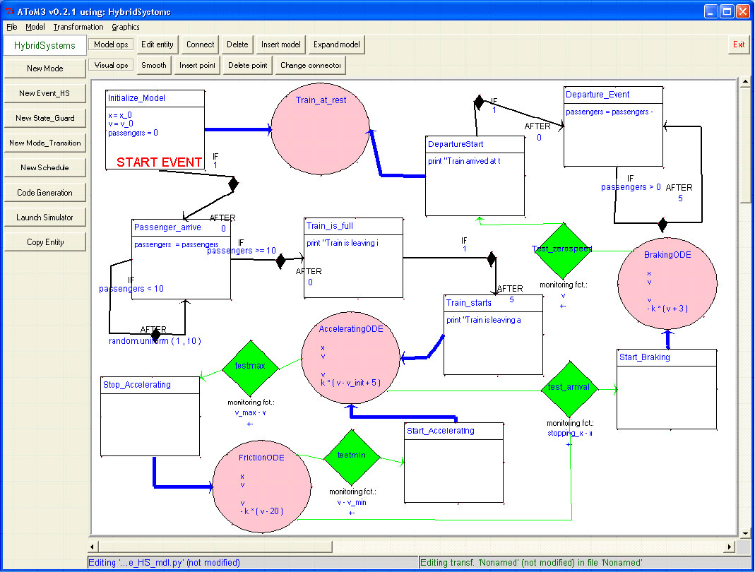
Train Example
This was the main example that Hans had used to motivate the requirements
for the 522 Simulator, since it contained everything that was wanted for
the simulator: discrete behaviour, continuous behaviour and event
scheduling. The model built with the HS formalism is shown in
figure 7. The file containing the model is
models_HS/TrainSchedule_HS_mdl.pyc.
This is a model of a train which travels in one dimension, and which
takes passengers at a station and then leaves them at another station.
The starting situation is the train at rest at the first station,
waiting for 10 passengers to arrive. The passengers arrive
at a random time interval between 0 and 10 seconds (using
the function random.uniform). When the 10 passengers have
arrived, the train departure is scheduled in 5 seconds. The train
then starts accelerating. Its speed is controlled by bang-bang
control between vmax and vmin (when it is not
accelerating, air resistance and friction makes it
decelerate (this is encoded in the Mode FrictionODE)).
When the train reaches the position stopping_x,
it starts braking in order to be at rest when reaching
the second station. When it becomes at rest, the passenger
starts to leave at constant interval of 5 seconds.
All of this can be easily understood by following carefully
the model in figure 7.
Figure 7: Train example in HS. The model can seem pretty
complicated at first sight, but by starting from the Start_Event
and following the connections, the semantic can be inferred quite
easily. Notice the use of the
random.uniform function in a Schedule relation for the
Passenger_arrive Event_HS. This can be done because the
random module was given in the Import_Modules list
in the global attributes of the model.
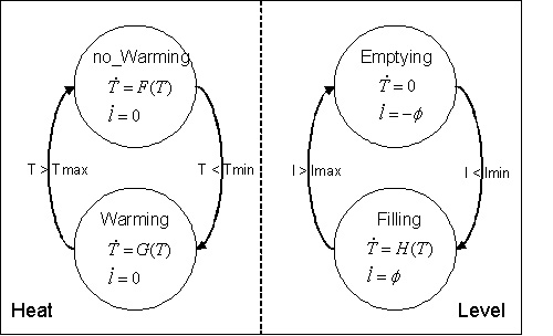
Heating Pot
This is an example that Hans had used extensively in talks he gave about
the use of multiple formalisms. The detailed description of
the heating pot example can be found in p.14 of his
notes about the Modelling and Simulation Process for the course 308-522A.
Briefly, it represents a pot of water which can be warmed at the rate of W Joules
per second, and filled with water at temperature Tin at the rate of phi cm/s
(represents the level variation). The temperature of the pot needs to be kept
between two thresholds, as well as its level. This is why you have four
monitoring functions. This model is a good example of how you can use
local variables, and how you can use parameters to change the state of a system
(since at first sight, we could wonder where is the discrete change in this
model because there is only one Mode). The main differential equation is
dT
dt
=
1.0
l
(heat - phi ·filling ·(T - Tin))
where
heat =
W
c ·rho ·A
where c is the specific heat of the liquid, rho is its density, A is the
cross-section surface of the pot, l is the level of the liquid, filling
is a parameter set to 1 when filling, 0 when emptying the pot. Also, you
can notice the line 'self.W_init = W' in the action code
of the Initialize_Model event. This defines a variable
W_init which is used to remember what was the initial
heating rate. Then, this rate can be set to 0 when the heating
is stopped (in event stopWarming) or reset to its initial
value when the heating is restarted (in event startWarming).
This example also demonstrates the poor display feature that AToM3
has for now: the equations are not displayed completely. Another
way to build this model will be explained in section 4.5.
We describe in this section how to generate code compatible with the 522 Simulator
from a model built with AToM3 with the Hybrid System formalism.
This could be done in a visual way using a graph grammar transformations
with AToM3, doing pattern matching for the structure of the model and
generating corresponding code in a file. A tutorial on how to work
with graph grammars with AToM3 (also written by Marc Provost) is given
here.
But because there are a lot of global preprocessing to do on the model for
this task, and also a preferred order for the code production, the paradigm of
pattern matching is not necessarily easy to use for this task. For this reason,
I have only used the graph grammar utility of AToM3 in order
to facilitate the interfacing of my code generator with the model created in
AToM3, but I haven't used any of its pattern matching ability. So I only
put all the Python code of my code generator in the 'initial action' attribute
of a graph grammar. This graph grammar model is given in
HS_atom3TO522Simulator_GG_mdl.py11, with
the executable code for the graph grammar given in
HS_atom3TO522Simulator.py.
The code for the initial action was simply taken from the file
code_for_codeGen/gen522Code.py, and is explained in the next section.
There are two main tasks that I needed to accomplish to build a code
generation tool for HS in AToM3. The first one was to understand well
the structure of the model in the HS formalism, compare it with the
one needed for the 522 Simulator and then create a corresponding
code generation algorithm. This will be explained in section 4.3.1.
The second task was to implement this algorithm,
and to do this, I needed to find how to navigate through the AToM3
data structures and how to get information about the model. This will be
explained briefly in section 4.3.2.
A HS model file for the 522 Simulator must contain the following
[see the file
PoolTable.py for a commented standard example of such a model file]:
One class per continous mode (they are subclasses
of Model.FirstOrderDEs), which gives the specifications
of the ODE in each mode.
One model class (subclass of Model.Model) which does the following:
defines the list of state variables and parameters using the
attributes modelvarnames and params respectively;
defines the start function which is used to
initialize the model: it initializes the state variables
using certain parameters as initial conditions; it initializes
the diffeqs variable to the starting ODE class (possibly an empty ODE);
it initializes the zerocrossingfuncs variable to
the current list of zero-crossing functions in use;
defines all the zero-crossing functions needed in the model;
defines all the event handlers functions needed in the model.
With this structure in mind, here is the code generation algorithm:
Prompt user for the file name of the generated file
Write header, doc and import statements [using information from the global attributes
in the model such as the Import_Modules list]
For each Mode in the model, write an ODE class:
Write __init__:
Write its signature: probe ODEs and Local_Parameters
to see what variables and global parameters were used
Build varnames and varderivs
Initialize parameters (local AND global used) [use the expressions
in Local_Parameters for the local parameter; in
Parameters_List for the global ones]
For each ODE variable, write the derivative functions [use RHS of
ODEs]
Write the model class:
Write __init__:
Signature: global parameters with default value [from
Parameters_List]
Initialize global parameters; and set variables to 0.0
Write the start() function:
Find the Start_Event and just schedule it from this function
For each Event, write an event handler function definition:
Write the Action_Code
If there is a Mode_Transition, then
Assign the new Mode ODE instance to diffeqs
For each State_Guard connected to this new Mode, add
it to zerocrossingfuncs
For each Schedule connection; write an if test using
Condition and put in its body the scheduling of the event
which is connected to it, in Schedule_in seconds
For each State_Guard, write the zero-crossing function definition
[using Monitoring_fct expression]
The implementation of this algorithm wasn't too hard, but was very time consuming because
there were lots of little details to consider and also because I needed to find out
how to navigate through the AToM3 data structure (see section 4.3.2).
The (nicely commented) code for the code generation is given in
code_for_codeGen/gen552Code.py. This uses some utility functions from
code_for_codeGen/codeGenTools.py, namely some string functions which permit
to have a nice generated code layout (with lines no longer than 100 char), and
an indent class which helps with the indentation of the generated code.
As mentioned in the previous section, the code generation was launched using a
graph grammar.
Some validation of the model is also done while generating code. Conceptually,
this should really be done at the modelling level (and not when generating code),
but for a prototype, the validation was done wherever it was possible to do some
(i.e. I haven't made sure that everything in the model was validated, but when I
had the possibility to validate something, I used this opportunity). The only
validation which is done at the modelling level automatically by AToM3
is the cardinality checking for the connections between objects; I haven't put
any constraint in the meta-model of the HS formalism. Here are the few checks
that are done while generating code:
Check that the variables on the LHS of the ODE declarations (in ODEs)
are in the Model_variables list;
Check that ODEs and Local_Parameters are list of tuples;
Verify that there is exactly one Start_Event;
Delete unused events and inform the user about this (unused events are
events which don't have any incoming connections);
Examples of generated code for HS models are given in the directory generated_models;
the HS models are given in the directory models_HS.
There are really only a few commands needed for our purpose, to navigate through the
AToM3 data structure. But finding them for the first time is not easy, so that's
why I will document them here. First of all, I made heavy use of Juan's API description
which can be found
here.
So here are the necessary commands:
First of all, we need to get an hold on an AToM3 instance from the
graph grammar; you can access it using: self.rewritingSystem.parent
when you are defining a GG rule. Say we call it atom3 for the remainder
of this section.
You can now access the root of the abstract syntax graph for the model (ASG),
with atom3.ASGroot. All the global attributes of the
model are stored in it. You can obtain the value
of an AToM3 attribute with getValue(). For example, to get
the author name of the model, you can do atom3.ASGroot.Author.getValue().
We can obtain the list of nodes in the model graph by accessing
atom3.ASGroot.listNodes, which is a dictionary which contains lists of pointers
to each node (indexed by node type). For example, you can access all the Mode
nodes in the model with atom3.ASGroot.listNodes['Mode']. This is used to
traverse the whole model. The attributes for a specify node is simply stored
in this node. For example, can get the name of the first Mode with
atom3.ASGroot.listNodes['Mode'][0].Name.getValue().
To find the connections of one node, you use
<node>.in_connections_ or out_connections_ which are lists
of pointers to incoming connected nodes and outgoing connected nodes, respectively.
Note that a relationship is also considered as a node, so you usually
have to pass through two connections before getting to a new node of the same
type. To check for the type of a node, you use the getClass() function.
For example, here is a little code excerpt which would find the Mode connected
to an event through a Mode_Transition:
# assume event contains an Event_HS node
for node in event.out_connections_:
    if node.getClass() == 'Mode_Transition':
        # Note that this node is a RELATIONSHIP;
        # Also, by the cardinality check of AToM3,
        # we know that only one Mode can be connected
        # (outgoing) from a Mode_Transition,
        # so we can simply take the first one in the list.
        mode = node.out_connections_[0]
        return mode
A final important thing to know: the return values of boolean
and enum types are not necessarily standard.
<ATOM3Boolean>.getValue() will return
(<display text>, <value>). <ATOM3Enum>.getValue()
will return a tuple with the list of possible values as the first element,
and the index of the current value of the enum as the second element.
There is now a bit more documentation about AToM3 on the web. A good example
of how to navigate through the AToM3 data structure is given
here, in a file written by Hans Vangheluwe for an assignment about Causal Block Diagrams
for the Modelling and Simulation
course at McGill.
The code for the new 522 Simulator (new modelling environment + DASRT included)
can be downloaded from
here. To make it work, you will need
AToM3. It is really easy to install AToM3: simply
extract it somewhere and run it with Python! Extract HybridSystems.zip
somewhere (preferably in the AToM3 directory), and then add its path
to the 'Path Directories' field in the options of AToM3 (this can be found
from file|options in the menu). You can then start modelling in the
Hybrid Systems formalism by loading the meta-model HybridSystems.py.
The button 'Launch Simulator' launches the simulator given in the directory
Simulator522. At first, this directory will contain the new simulator
which includes the new solvers (cEuler, fEuler, f2pyEuler, DDASSL and DDASRT -
see section 3.6. To make this simulator works, you will need
numpy, and you could
also need to rebuild the solvers (see section 3.6).
In case you don't want to do that, the folder Simulator_minimal
contains a minimal version of the simulator, which doesn't use any
of the new solvers (and which is more than enough for anything you want
to do, since the new solvers are only there to show that they work...).
To use this solver instead, simply rename its directory to Simulator522.
To simulate your HS models, you first have to generate code using the
'Code Generation' button. Then, you can load the generated file in
the simulator as a model file.
Appendix E contains a list of all the important files
and directory found in the HybridSystems directory.
Now that we have a graphical modelling environment for Hybrid Systems,
it is a lot easier to study what could be the best formalism to model
them. One path that could be investigated would be to use statecharts
instead of simple FSA.
The need for statechart became evident when I tried to remodel the
Heating Pot example (figure 8) by using
different Modes instead of changing the parameter in the ODE. The problem
was that because the emptying/filling behaviour is concurrent with
the warming/not_warming behaviour, we obtain a combinatorial explosion
of states. The number of needed Modes is not 2, but 4, and the number
of state guards passes from 4 to 8. Indeed, due to bugs in AToM3,
I have never completely succeeded to rebuild the model in this way; there
were so many entities to build that it always bugged before I finished!
Statecharts would solve this problem since it has support for concurrent
states, thus avoiding the combinatorial explosion when there are
independent transitions characterizing a system. The Heating Pot model
using statecharts is shown in figure 9.
The question that one could ask then is what would be the semantic of
two concurrent modes. Well,
it could simply be that the RHS of the ODEs for the same variable name
would be added. For example, if the system was in the no_Warming state
and in the Filling state in figure 9, then the ODE for T
would be:
dT
dt
=
F(T)fromno_Warmingstate
+
H(T)fromFillingstate
This would be meaningful if the contributions could be simply added, but this
is often the case in Physics where we have the superposition principle.
Apart avoiding the combinatorial explosion, this way of modelling has the merit
of clearly showing the concurrent nature of two different characteristic
of the system (here, the level change vs. the heating).
Figure 9: Heating Pot model using statecharts
Another thing we have found this summer is how to use DASSL (or DASSRT)
to do acausal modelling, that is, to model physical systems without
assigning any causality (like is done in the modelling language
Modelica). For example, we would like
to model a (electric) capacitor with the equation C ·dv/dt - i = 0
without having to say if it is i (the current) or v (the voltage)
which is known. Depending of what happens around the capacitor, we would
like sometimes to drive with i, other times (maybe in the same simulation
run) with v. This can be done in DASSL by giving as the residual equation: RES[1] = C*YDOT[1]-Y[2]
(assuming Y[1] = v and Y[2] = i) with the following constraint which
will drive the desired variable: RES[2] = Y[f.index] - f(t)
Now, f could be a Python object which would represent which variable
is driven (f.i would be set to the index of this variable in Y),
and f(t) would call the appropriate driving functions. The beauty
of this is that f could be changed at run-time. This would truly
permits acausal modelling, and would be useful when we will want to extend
the Hybrid Systems formalism with input/output support.
The goal for me this summer was to get a feel for
multidisciplinary research, and this has been done! I have
learned how to do extension and embedding for Python, how to mix
C and Fortran (and at the same time, the mysteries of gcc and
dynamically linked libraries). I became familiar with the
world of scientific computing on the net (netlib, SciPy, SciLab, etc.).
I learned about the code development world; how to find info about bugs;
when to ask questions, etc. I learned how to use GDB (in details).
All those skills will be very useful to reuse all the scientific
libraries which are present on the web.
Regarding the modelling and simulation of Hybrid Systems, it has been shown how
AToM3 could be used to build a powerful modelling
environment, quickly. The 522 Simulator has been improved with a GUI,
as well as with the addition of the DASRT solver. The task of extending
Python with Fortran code has been very instructive, and quite useful,
as the several questions I received about it can show. Several
improvements for the modelling and simulation of Hybrid Systems
were suggested. I will discuss them in next section.
I will build the next generation of the 522 Simulator as a project this semester
in the course Modelling and Simulation at McGill University.
The main things to do will be to redesign the core of the 522 Simulator, so that
the modelling and the simulation components are clearly independent.
Also, the support of DAEs should be added.
Other improvements that could be brought are the following:
The addition of an algebraic solver so that equations (to be solved)
could be put in the action code of an event (this would be quite useful
for the initialization of the state variables after a mode
transition; e.g., we could demand that the variables respect
conservation of energy and momentum, and the simulator would find
by itself the correct values under these constraints).
Nice documentation features so that the user could check
the meaning of each variable in the simulation environment.
Adding units/dimensions support: this would permit
dimensional analysis (and verification) at the modelling level.
Modelling with Statecharts instead of FSA (as was mentioned
in section 4.5).
Adding the support for constrained variables and the
connection of components (using input/output formalism).
This would permit to model driven systems in a modular way;
and also to do acausal modelling.
I would like to thank sincerely Hans Vangheluwe for all the guidance he
has provided me with this summer. He was always available to discuss
about Life, Universe and Everything, and our 1 hour meetings often
transformed into 5 hours meeting... I would also like to
thank Marc Provost and Ernesto Posse for their useful help about AToM3,
Pearu Peterson for his help about f2py (and to have developed such
a useful tool!) and Juan Jaramillo for having built (with Hans) AToM3,
a tool which will permit the MSDL to take over the world! ;-)
The problem that you may face when you want to debug a shared library
with GDB is that the symbol table of the shared library is not loaded
until it is imported. This means that you can't set breakpoints before
it is imported. But if it crashes after it gets executed, how are you
supposed to debug it if you can't stop it before it crashes? The solution
resides in the magical SIGINT interrupt: CTRL-C which permits to break
the execution of the program at any time. So the idea is to have your program
stop just after it has loaded the shared library, but before it
executes them. For example, in my Python extension modules, the execution
of the test modules was always done using a run method. As a result,
when I imported the module, the shared library were not executed: they were
only loaded. This permitted me to do the following steps to debug the
shared library:
Compile your shared library with the -g option.
In case you won't have an obvious place where you will have time
to press the CTRL-C command after the loading of the library
but before its execution, put a sleep statement in
the source code where you want to break it.
Run python under gdb (with a command like gdb -args python2.2 <test_module> for Unix).
Do run to start the execution of the import statement; if you were importing
shared libraries in the test_module, now they should be loaded.
When you reach the sleep point, send a SIGINT interrupt (CTRL-C)
to switch control back to gdb.
Look with info shared to see if the symbols have been read
(look at the 'syms read' column); if they haven't been read,
then you can reload them with the command share <file>.so.
Now you can add the breakpoints as usual into your shared library, and start debugging it.
B Source files related to the Euler solver written in C
B.1 Euler.c: source code for a Euler solver written in C
/* Written by Simon Lacoste-Julien on 2002/07/23 */
/* This is a test for Python Extension.
I'm implementing the Euler solver used in the 522 Simulator.
Interface of use:
>>> import Euler
>>> newx = Euler.step(f,x,t,delta_t) # as before!!!
Where f is an array of (derivative functions) [of the form g(x,t)], x is initial array of values,
t is time, and delta_t is step length (both are double).  That's it!
Magic of Python API... */
/* newx = Euler.step(f,x,t,dt) will simply yield:
newx = x + f(x,t) * dt
*/

#include <Python.h>

/***** 2) Module method definition ********/
static PyObject*
step(PyObject* self, PyObject* args) {

    PyObject* f_array = NULL;       /* will hold f */
    PyObject* f_call = NULL;        /* will hold f[i] (to be called) */
    PyObject* x_array= NULL;        /* will hold array x */
    PyObject* newx = NULL;          /* will hold result (array)*/
    PyObject* xObject = NULL;       /* will hold Python x[i] */
    PyObject* arglist = NULL;       /* will hold arguments for call of f[i] */
    int length;             /* size of f and x */
    int i;                  /* array index */
    double x, x2, t, delta_t;   /* x will hold x[i], x2 will hold result of computations  */

    if (PyArg_ParseTuple(args, "OOdd",
            &f_array, &x_array, &t, &delta_t) == 0) {       /* converts Python -> C */
        /* setting error message: */
        PyErr_SetString(PyExc_RuntimeError, "Wasn't able to parse args for Euler.step fct.");
        return NULL;        /* when returning null, you raise an exception */
    } else {
        Py_INCREF(f_array);
        Py_INCREF(x_array);
        if((PyList_Check(f_array) && PyList_Check(x_array)) == 0) {
            PyErr_SetString(PyExc_TypeError, "Error: f or x weren't list!");
            goto error;
        }

        length = PySequence_Length(f_array);    /* assume x_array has same length... */
        newx = PyList_New(length);              /* initializing the return array */
        Py_INCREF(newx);

        /****** Euler loop ********/
          for(i = 0; i < length; i++) {
            Py_XDECREF(f_call);
            Py_XDECREF(xObject);
            f_call = PyList_GetItem(f_array, i);
            xObject = PyList_GetItem(x_array, i);
            Py_INCREF(f_call);
            Py_INCREF(xObject);

            x = PyFloat_AsDouble(xObject);      /* set x = (double) xObject */

            /* evaluating f[i](x,t) : */
            Py_XDECREF(arglist);
            arglist = Py_BuildValue("(O,d)", x_array, t);   /* building (x,t)  NOTE: x is a vector! */
            Py_INCREF(arglist);
            x2 = PyFloat_AsDouble(PyEval_CallObject(f_call, arglist));  /* x2 = f[i](x,t) */

            /* Euler computation: */
            x2 = x + delta_t * x2;

            /* set result[i] = x2 :*/
            PyList_SetItem(newx, i, Py_BuildValue("d", x2));
        }

        /* cleaning pointers: */
        Py_XDECREF(f_array);
        Py_XDECREF(f_call);
        Py_XDECREF(x_array);
        /* not doing it on newx since we're returning it */
        Py_XDECREF(xObject);
        Py_XDECREF(arglist);

        return newx;
    }
    error:
        /* cleaning memory: */
        Py_XDECREF(f_array);
        Py_XDECREF(f_call);
        Py_XDECREF(x_array);
        Py_XDECREF(newx);
        Py_XDECREF(xObject);
        Py_XDECREF(arglist);

        return NULL;        /* this raises exception */
}

/***** 3) Registration table  **************/
/* this gives the association between the function NAMES (to be used
in Python namespace) to function pointers (addresses) giving the C implementation */

static struct PyMethodDef Euler_methods[] = {
    {"step", step, METH_VARARGS, "Implements Euler solver."},
    /* method name, C func ptr., method of calling fct, method doc */
    {NULL, NULL, 0, NULL}                    /* end of table marker */
};

/***** 4) Initialization function for the module *****/
/* this is called the first time the C module is imported in Python;
it builds the Module's attribute dictionary from the registration
table and create an entry for the C module on the sys.module table */
/* name of fct matters: should be init<moduleName> */
void initEuler() {
    (void) Py_InitModule("Euler", Euler_methods);   /* module name, table ptr */
}
# This is a test script for the Euler solver written in C
# To use it, simply do
# >> import test
# >> test.run()

# defining the derivative functions:
def f1(x,t):
    return x[0]*x[1]

def f2(x,t):
    return -x[0]*t

L = [f1,f2] # this is the array of derivatives (represents the ODE)

# setting the initial conditions:
x = [1,2]
t = 1.0
dt = 5.0

# importing the extension module:
import Euler # we need Euler.so or Euler.pyd in the path...

# the testing routine:
def run():
    newx = Euler.step(L,x,t,dt) # testing Euler extension!
    print "Euler.step(f,x,t,dt) with f = [x[0]*x[1], -x[0]*t], \
        x =", x, "t =", t, "and dt =", dt
    print "yields newx = ", newx
    print "This should be [11.0, -3.0] if everything works."
C Source files related to the Euler solver written in Fortran
C.1 Euler.f: source code for the Euler solver written in Fortran
C       Written by Simon Lacoste-Julien 02/7/29
C       This is a test to implement Euler function with call-back
C       mechanism in Fortran, to extend Python...
C
C EULER(N, fun, x, t, dt, newx)
C   - N is size of array input (x)
C   - fun is the ODE function - it's really an array of function; but this will
C     be taken care of in the python code: it will be called as follows
C        fun(N,i,x,t, result) where i will be the index of which function
c           to evaluate (i starts at 0 in Python)
C        x will be vector
C        t will be scalar
C        result will hold result
C   - x is state vector
C   - t is time (double)
C   - dt is time step (double)
C
        SUBROUTINE EULER(N, fun, x, t, dt, newx)
            EXTERNAL fun
            INTEGER N
            DOUBLE PRECISION x(N), t, dt, newx(N)
            DOUBLE PRECISION res

            DO 10 i = 1, N
               CALL fun(N,i-1,x,t, res)
               newx(i) = x(i) + dt * res
 10         CONTINUE

        END SUBROUTINE EULER
C.2 fEuler.c: source code for the C wrapper for fEuler.f
/* Written by Simon Lacoste-Julien on 2002/07/29 */
/* This is a test for Python Extension and fortran linking
I'm implementing the Euler solver used in the 522 Simulator, but using fortran code
Interface of use:
>>> import fEuler
>>> newx = fEuler.step(f,x,t,delta_t) # almost as before!
The difference is that f is no more an array of (derivative) functions, but it
is called as f(i,x,t) where i will be the index of the derivative required...
x is initial array of values,
t is time, and delta_t is step length (both are double).  And the return value
is a simple double.
*/

#include <Python.h>

/* SUBROUTINE EULER(N,fun(N,i,x,t),x,t,dt,newx) imported from Fortran: */
extern void euler_(int* N, void (*fun)(int* N1, int* i, double x1[], double* t1, double* res),
            double x[], double* t, double* dt, double newx[]);
/* notes: 1) euler_ is in lower-case and have added '_' for the name compatibility with Fortran
          2) all the arguments are passed as pointers, since Fortran pass arguments by reference
      and not by value... */

/***** Callback function interface between C and python for the derivative function: ************/
/* CALL-BACK POINTER: */
static PyObject* funPython = NULL;  /* this will hold the function passed by Python; it is GLOBAL! */

/* CALL-BACK FUNCTION WRAPPER: */
static void callBack(int* N, int* i, double x[], double* t, double* res) {
  PyObject* arglist = NULL;
  PyObject* x_python = NULL;
  int j;

  /* arguments translation: */
  x_python = PyList_New(*N);
  Py_INCREF(x_python);
  for(j = 0; j < (*N); j++) {
    PyList_SetItem(x_python, j, Py_BuildValue("d", x[j]));
  }

  arglist = Py_BuildValue("(i,O,d)", *i, x_python, *t);    /* building (i,x,t)  NOTE: x is a vector! */
  Py_INCREF(arglist);
  *res = PyFloat_AsDouble(PyEval_CallObject(funPython, arglist)); /* *res = (double) funPython(i,x,t) */

  /* memory cleaning: */
  Py_DECREF(arglist);
  Py_DECREF(x_python);

  return;
}


/***** 2) Module method definition ********/
static PyObject*
step(PyObject* self, PyObject* args) {

  PyObject* x_python = NULL;        /* will hold array x in Python */
  PyObject* newx = NULL;          /* will hold result (array) in Python */
  PyObject* xObject = NULL;       /* will hold Python x[i] */
  double* x_array;                /* array to hold values of x in C format */
  double* workArray;              /* array to hold new values of x in Fortran call  */
  int length;             /* size of x */
  int i;                  /* array index */
  double t, dt;

  /* getting arguments from python: */
  if (PyArg_ParseTuple(args, "OOdd",
               &funPython, &x_python, &t, &dt) == 0) {       /* converts Python -> C */
    /* setting error message: */
    PyErr_SetString(PyExc_RuntimeError, "Wasn't able to parse args for Euler.step fct.");
    return NULL;        /* when returning null, you raise an exception */
  } else {
    Py_INCREF(x_python);
    Py_INCREF(funPython);
    if(PyList_Check(x_python) == 0) {
      PyErr_SetString(PyExc_TypeError, "Error: x wasn't a list!");
      goto error;
    }

    /************ converting Python to C/Fortran: **************/
    length = PySequence_Length(x_python);
    x_array = calloc(length, sizeof(double));    /* x array in C */
    workArray = calloc(length, sizeof(double));  /* to be used by Fortran code */

    /* initializing x_array: */
    for(i = 0; i < length; i++) {
      Py_XDECREF(xObject);
      xObject = PyList_GetItem(x_python, i);
      Py_INCREF(xObject);
      x_array[i] = PyFloat_AsDouble(xObject);
    }

    /* CALLING Fortran code: */
    euler_(&length, callBack, x_array, &t, &dt, workArray);

    /************* translating result to Python *****************/

    newx = PyList_New(length);              /* initializing the return array */
    Py_INCREF(newx);
    for(i = 0; i < length; i++) {
      PyList_SetItem(newx, i, Py_BuildValue("d", workArray[i]));
    }

    /* cleaning memory: */
    Py_XDECREF(x_python);
    /* not doing it on newx since we're returning it */
    Py_XDECREF(xObject);
    Py_XDECREF(funPython);
    free(x_array);
    free(workArray);

    return newx;
  }
 error:
  /* cleaning memory: */
  Py_XDECREF(x_python);
  Py_XDECREF(newx);
  Py_XDECREF(xObject);
  Py_XDECREF(funPython);

  return NULL;        /* this raises exception */
}

/***** 3) Registration table  **************/
/* this gives the association between the function NAMES (to be used
   in Python namespace) to function pointers (addresses) giving the C implementation */

static struct PyMethodDef fEuler_methods[] = {
  {"step", step, METH_VARARGS, "Call Fortran Euler Solver."},
  /* method name, C func ptr., method of calling fct, method doc */
  {NULL, NULL, 0, NULL}                    /* end of table marker */
};

/***** 4) Initialization function for the module *****/
/* this is called the first time the C module is imported in Python;
   it builds the Module's attribute dictionary from the registration
   table and create an entry for the C module on the sys.module table */
/* name of fct matters: should be init<moduleName> */
void initfEuler() {
  (void) Py_InitModule("fEuler", fEuler_methods);   /* module name, table ptr */
}
C.3 setup_fEuler.py: python script to build extension module fEuler
# written by SLJ 2002-8-28
# took model from http://www.python.org/doc/current/ext/building-on-unix.html
# To use it on my Windows XP (with mingw gcc compiler):
# python setup.py build --compiler=mingw32
# It uses the library libEuler.a

from distutils.core import setup, Extension

module1 = Extension('fEuler',
                    libraries = ['Euler'],
                    library_dirs = ['./'],
                    sources = ['fEuler.c'])

setup (name = 'fEuler',
       version = '1.0',
       description = 'This a Euler solver implemented in Fortran',
       author = 'Simon Lacoste-Julien',
       author_email = 'simonlacoste@videotron.ca',
       url = 'http://moncs.cs.mcgill.ca/MSDL/people/slacoste/',
       long_description = '''
This is really a Euler solver implemented in Fortran!
''',
       ext_modules = [module1])
C.4 test_fEuler.py: a test script for the fEuler module
# This is a test script for the Euler solver written in Fortran
# To use it, simply do
# >> import test_fEuler
# >> test_fEuler.run()

# defining the derivative functions:
def f1(x,t):
    return x[0]*x[1]

def f2(x,t):
    return -x[0]*t

L = [f1,f2] # this is the array of derivatives (represents the ODE)

# importing the extension module:
import fEuler # we need fEuler.so or fEuler.pyd in the path...

# we define here a routine similar to the one that will be
# used from the 522 Simulator
def step(f,x,t,dt):
    # we need to change the way f is called (to be consistent with
    # new interface of the solver
    def fun(i,x1,t1):
        return f[i](x1,t1)
    return fEuler.step(fun,x,t,dt)

# setting the initial conditions:
x = [1,2]
t = 1.0
dt = 5.0

# the testing routine:
def run():
    newx = step(L,x,t,dt) # testing fEuler extension!
    print "step(f,x,t,dt) with f = [x[0]*x[1], -x[0]*t], x =", x, "t =", t, \
          "and dt =", dt
    print "yields newx = ", newx
    print "This should be [11.0, -3.0] if everything works."
2DASSL:
Differential Algebraic Systems Solver Library
3The first
'd' is to indicate that the code is using
double precision numbers; sdassl.f will represent the single precision
version.
4
This has been a major source of frustration for me during this project, as
the basic commands to use f2py described in the user guide
were completely obsolete. The general information about f2py
given in the user guide is still correct [I think], though.
5If we want to be rigorous, it could happen that this chain
of meta-levels would never end (and this is reminiscent of meta-theory chains that happen
also in the rigorous definition of theories in logic...).
7``Event_HS'' was used instead of ``Event'' for the name
of this entity in order to avoid name conflict with Tkinter (used internally by AToM3).
8Notice the AToM3 naming
convention: the name of the model being built (HybridSystems)
followed by the formalism
in which it is built (ER) followed by mdl.py.
9Here, entity
means simply ``object which can be added in the model''. So it can be either
an entity from ER or a relationship from ER. It is unfortunate that there
can be some ambiguity in the terminology of AToM3 since we have the button
``Edit entity'' which can be used to edit also relationships... It should
be clear from the context whether I use entity to mean entity from ER or general
entity.
10Note that AToM3displays lists (and tuple) as strings separated by |. For example,
(g, 9.8) is displayed as g|9.8|.
11The naming convention for a graph
grammar is <formalism>_<transformation name>_GG_mdl.py.
File translated from
TEX
by
TTH,
version 3.11. On 28 Oct 2002, 03:08.