CS-766B Assignment 2
Simon Lacoste-Julien
9921489
April 12 2003
Contents
1 Introduction
2 Part I: The Heat Equation
2.1 Gaussian Blur
2.2 Heat Equation Blur
3 Part II: The Geometric Heat Equation
3.1 Discretization
3.2 Level Curve Evolution
4 Images
4.1 Gaussian Blur
4.2 Heat Equation
4.3 Geometric Heat Equation
1 Introduction
I have used the Matlab image processing toolbox to implement this assignment.
The electronic version of my report with the images is available at
http://moncs.cs.mcgill.ca/MSDL/people/slacoste/school/cs766b/ass2.html.
2 Part I: The Heat Equation
2.1 Gaussian Blur
To implement the Gaussian blurring, I have used a square kernel with a radius of 4s
(i.e. a square with side of 8s+ 1), since the Gaussian is mostly zero
outside of it. I have convolved this kernel with the image using the filter2 function
of Matlab. The 2D kernel was of course:
|
K(x,y,s) = (2ps2)-1e-[(x2+y2)/(2s2)] |
| (1) |
with the origin placed at the center of the neighborhood. We note that the case presented
in the assignment was the heat equation in a unbounded domain with homogeneous
boundary conditions. So this means that the image needs to be embedded in a infinite domain
with zero intensity at infinity, and thus we simply padded the surrounding of the image with zeros
to do the convolution.
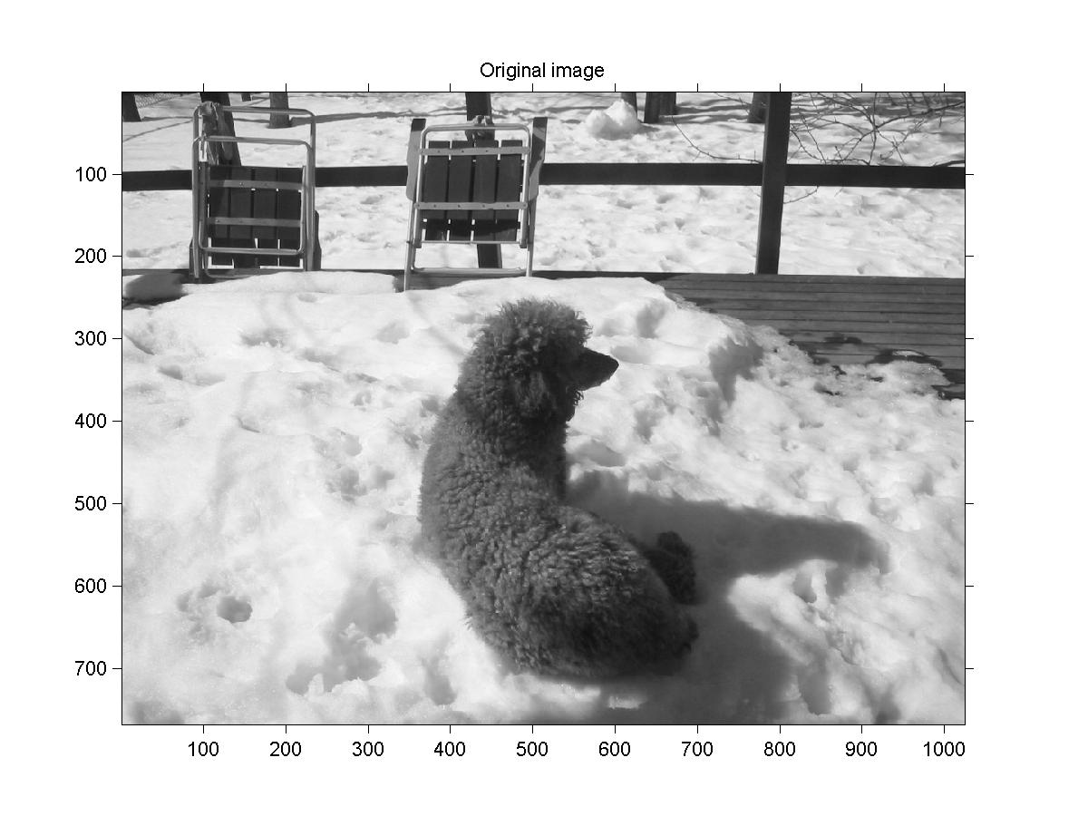
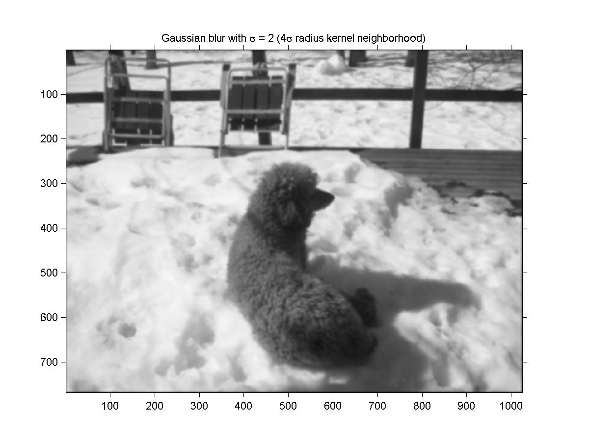
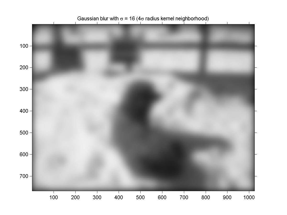
The original image is given in figure 1, with the blurred image with s = 2,
4, 16 pixels given in figure 2, 3 and 4 respectively.
2.2 Heat Equation Blur
To implement the derivatives of the heat equation, we used centered difference for the space derivatives
and forward difference (Euler integration) for the time derivative (formulas which can be derived
from manipulation of the Taylor series).
|
centered difference: f˘˘(x0) = |
f(x0+h) - 2f(x0) + f(x0-h)
h2
|
+ O(h2) |
| (2) |
|
forward difference: f˘(t0) = |
f(t0+h) - f(t0)
h
|
+ O(h) |
| (3) |
So the Euler integration step gives:
|
u(t+dt) = u(t) + dt·(uxx(t) + uyy(t)) |
| (4) |
We used of course a step size of h=1 since we only have intensity values at each pixel. An important
point to consider is which boundary value to use. The real problem is in an unbounded domain.
But to simplify the implementation, I have used a homogeneous boundary condition just outside of the
image (instead of at infinity). At the beginning, I hadn't really thought about it, I just padded
the image with zeros around it to compute the derivatives like I had padded with zeros to compute
the convolution. But as we'll see in the next section, this yields a major difference between
the convolution solution and the heat equation solution. In order to choose a step size for the
time integration, I have computed the difference of the solution obtained with two different step
sizes. To quantify the difference between two solutions, I have looked at the max norm (maximum
of the absolute value of the difference of the two images over all pixels) and the mean norm
(mean value of the absolute value of the difference). By computing the solution at t=2 (this was to
compare with Gaussian blur with s = 2) with dt = 0.2, 0.1 and 0.01, I obtained the images
I1, I2 and I3 respectively. Then I had the following results:
| max | mean |
|
|
| |I1-I2| | 0.0329 | 0.0013 |
| |I2-I3| | 0.0078 | 0.0003 |
Note that the image intensities were double floating point numbers between 0 and 1.
Since that the correction given by dt = 0.01
over dt = 0.1 was small, I used dt=0.1 for all my integrations (which gave a running time of roughly 15 seconds
on my home computer for each second of needed integration - and thus roughly 30 minutes to obtain an equivalent
blur than s = 16). To compare the heat equation solution with the Gaussian convolution, we use the equivalence
t = s2/2, and thus I have computed the solution for t=2, 8 and 128. To visualize the differences between
the heat equation solution and the Gaussian convolution, I have
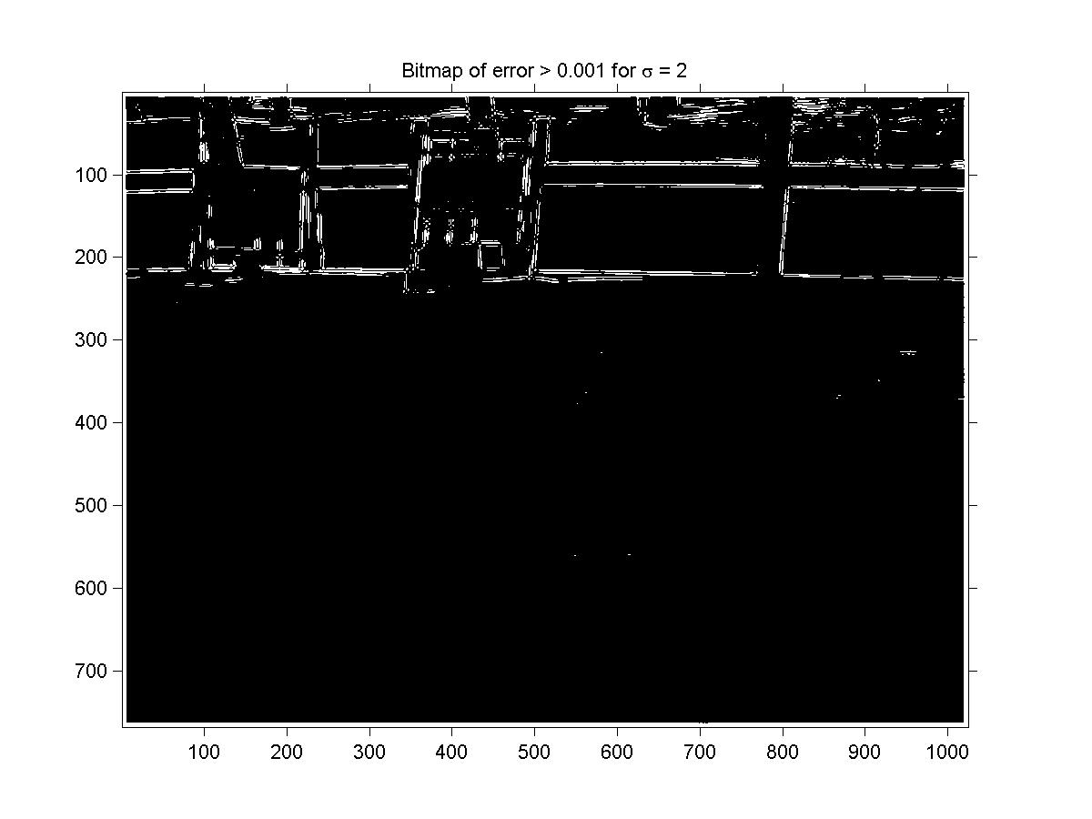
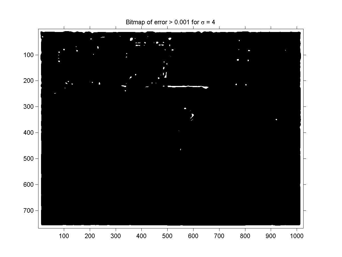
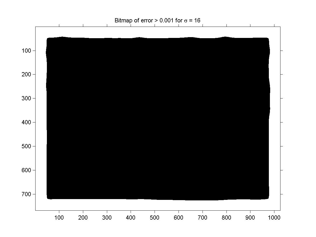
plotted a bitmap image of the pixels where the absolute difference is greater than 0.001 (0.1% error). These are plotted
in figure 5, 6 and 7. There were two main sources of the error:
- Discretization of derivative
- When the gradient of intensity is high, the error made with finite difference to
approximate the spatial derivative is the greatest. This is why at t=2 (figure 5) we see more error
close to the edges of the original picture. As the image gets smoother and smoother, this error averages out and
disappears completely as we can see at t=128 (figure 7).
- Boundary conditions
- This error is caused because I have used homogeneous boundary conditions at the boundary
of the image instead than at infinity. Ideally, I should have increased the domain of computation at the same time
as the value around the images became non-zero (instead of just keeping them to zero). But in my implementation,
the influence of the homogeneous boundary conditions spread gradually inside the image as time increased. This is why
you can see on the figures that the error region close to the boundary gets larger and larger (this is all we see
on figure 7 where t=128!).
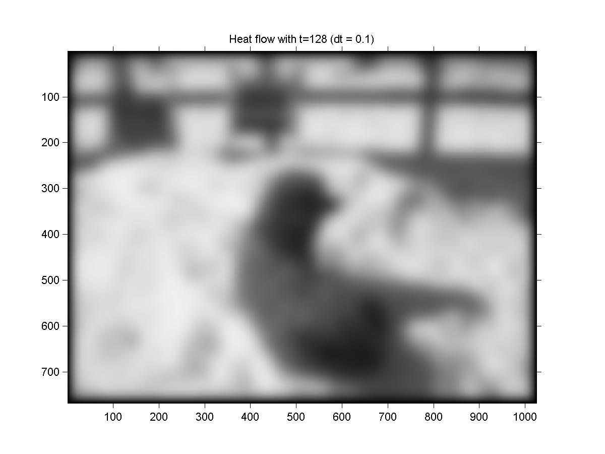
But apart those two sources of difference, the two results are pretty similar (in fact, you can't really distinguish
one from the other with the eye, except from the small black border at the boundary of the image which is more apparent
with the heat equation (because of the boundary conditions). See figure 8 for the result with t=128
using dt = 0.1.
3 Part II: The Geometric Heat Equation
Here, the heat equation becomes:
|
ut = |
uxxuy2 - 2ux uy uxy + uyy ux2
ux2 + uy2
|
|
| (5) |
A potential problem arises when Ńu = 0: the denominator vanishes. To see if there is some
way to extend the equation meaningfully in this case, we do some elementary manipulations to obtain:
|
|
uxx
x2+1
|
+ |
uyy
1+1/x2
|
- |
2uxy
x+ 1/x
|
|
| (6) |
where x = ux/uy. Now, depending what is the limiting behaviour of x = ux/uy as we approach
the point where Ńu=0, we will have different values for the RHS of (5). Probably
the appropriate way to implement this numerically would be to compute ux/uy for the points around
the pixel (4 values) and take their average or something similar. But this would complicate a lot the code,
so instead, I have just chosen the usual engineering approach of adding a very small number to the
denominator of (5):
|
ut = |
uxxuy2 - 2ux uy uxy + uyy ux2
ux2 + uy2 + e
|
|
| (7) |
so that we never divide by zero. At first sight, we could think that this would yield a somewhat different
flow than (6) because the latter can have a non-zero value (and big if uxx is big, for example)
even when Ńu = 0; whereas (7) will be zero when Ńu = 0. But, according to
Maxime Descoteaux, it was shown in [1] that the (weak) solution to (7) was the same
than the solution to (5) under some reasonable assumptions on the image. So let's say it will
be enough for this assignment!
3.1 Discretization
We can use the same finite difference equations given in section 2. We will need in addition two new formulas:
the centered difference for the first derivative, and for a mixed derivative:
|
ux(x,y) = |
u(x+h,y) - u(x-h,y)
2h2
|
+ O(h2) |
| (8) |
|
uxy(x,y) = |
u(x+h,y+h) - u(x+h,y-h) - u(x-h,y+h) + u(x-h,y-h)
4h2
|
+ O(h2) |
| (9) |
Again, I used Euler integration with time step dt = 0.1 and spatial grid h=1. I also used
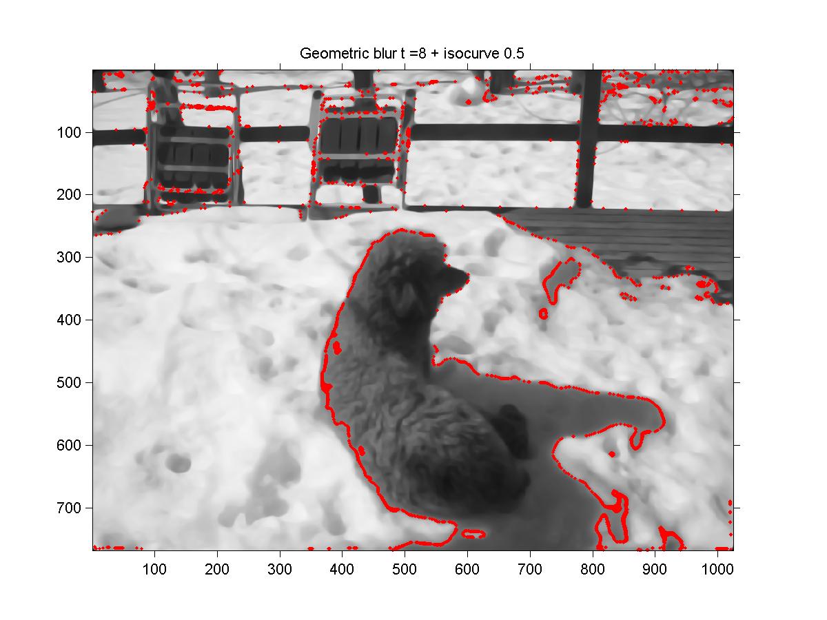
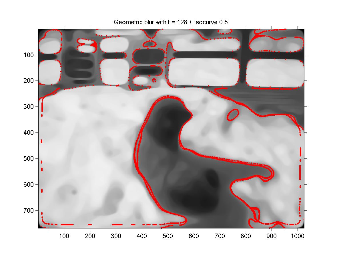
e = 1010 in equation (7). The results for t=8 and t=128 are given
in figure 10 and 11 respectively.
3.2 Level Curve Evolution
We can see the geometric heat equation (5) as the level set implementation of the
Euclidean Curve Shortening Flow:
where k is the curvature and N is the normal; i.e. we see the image as an embedding
of its level curves (curves of same intensity). So we would expect those (iso)curves to evolve
in the same way as they would under the curvature flow (i.e. stay smooth, preserve inclusion
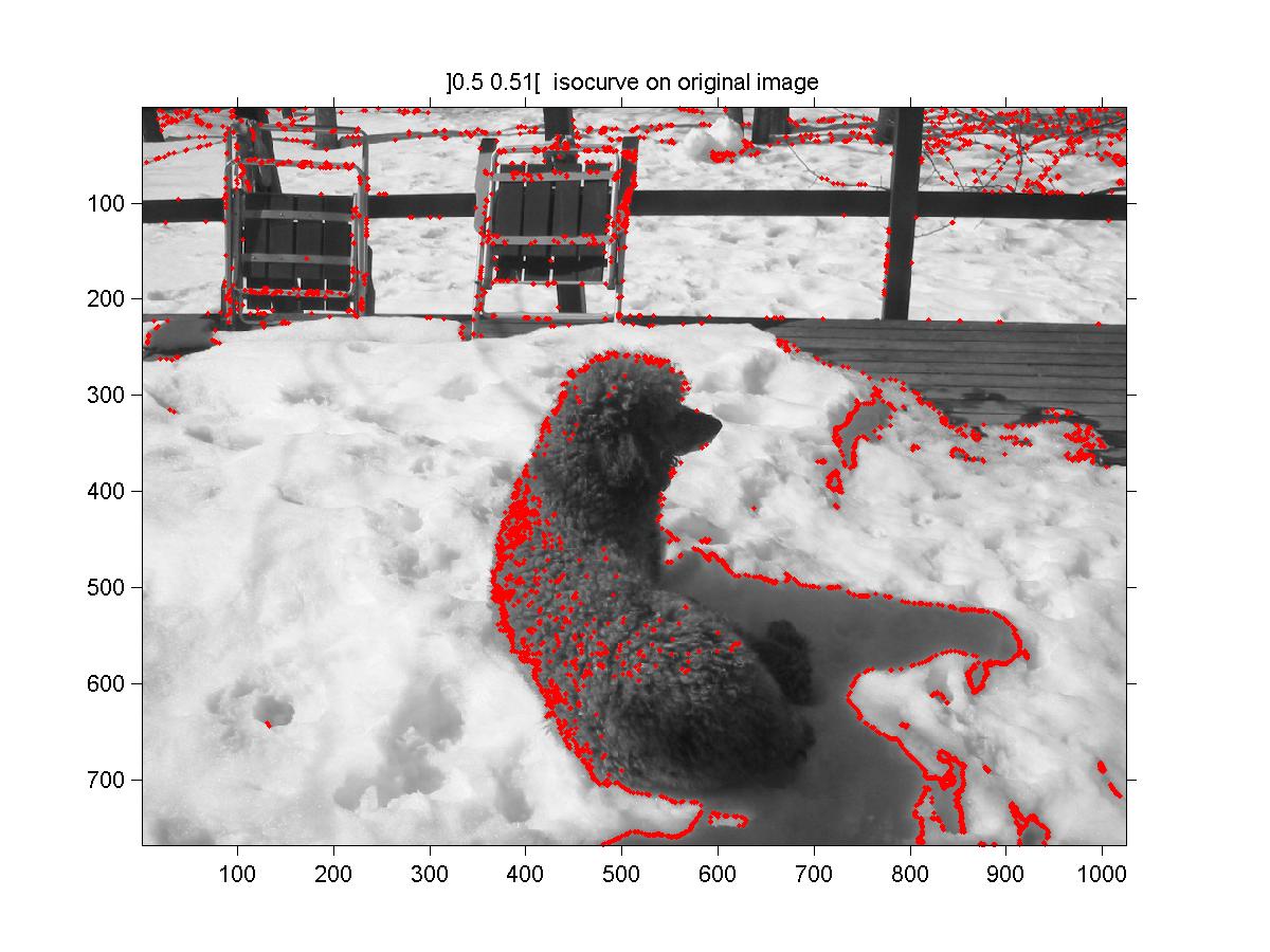
relationship and asymptotically become an elliptical point). Indeed, by plotting the isocurve
of the intensity between 0.50 and 0.51 on the image, we can see this somewhat. This is shown
on figure 9, 10 and 11, for t=0, 8 and 128 respectively.
At the beginning (figure 9), we can see several little points curve (especially on
the dog). Those will disappear (be smoothen) after the geometric flow (thus the geometric flow
blurs inside a region surrounded by an edge). By watching the curve
just to the right of the dog, we can see that it becomes an ellipse
as required (see figure 11). The fact that some curves are created in the last image
could probably be explained by discretization error (it is, after all 1280 steps). Since the curve
around the dog was at an important edge, it doesn't move much (since in geometric flow, the
edges are preserved). We can truly see on the last image (figure 11) that the
strong edges have been preserved (like the bars of the fence in the back; except at intersection
where some smoothing is done) by the geometric heat equation blur. So the blurring is truly along
edges and not across edges. On the other hand, the Gaussian blur blurs in all direction, and thus
it destroys edges (see figure 4).
4 Images
4.1 Gaussian Blur
 Figure 1: Original Image
 Figure 2: Gaussian blur with s = 2.
 Figure 3: Gaussian blur with s = 4.
 Figure 4: Gaussian blur with s = 16.
4.2 Heat Equation
 Figure 5: Bitmap of error threshold between Heat and Gaussian for s = 2. Here the
error is mostly due to the discretization error of the space derivative.
 Figure 6: Bitmap of error threshold between Heat and Gaussian for s = 4.
 Figure 7: Bitmap of error threshold between Heat and Gaussian for s = 16. Notice that all
the error is concentrated near the boundary, due to the discrepancy of the boundary conditions.
 Figure 8: Heat Equation with t=128. Notice the larger black boundary compared
with figure 4, due to the difference in boundary conditions.
4.3 Geometric Heat Equation
 Figure 9: Original image with isocurve between 0.50 and 0.51.
 Figure 10: Geometric blur with t = 8 and isocurve between 0.50 and 0.51.
 Figure 11: Geometric blur with t = 128 and isocurve between 0.50 and 0.51. Notice that
significant edges have been preserved (except that their intersection have been curved a little).
References
- [1]
-
L.C. Evans and J. Spruck, ``Motion of level sets by mean curvature, I'', Journal of
Differential Geometry 33, pp. 635-681, 1991.
File translated from
TEX
by
TTH,
version 3.11.
On 23 Apr 2003, 04:04.
