2.2 Mode Switching in the Hybrid Model

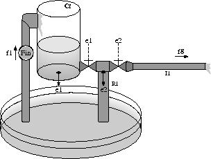
Discontinuous effects in physical system models occur when energy or power variables cross a certain threshold value. For example, a diode is modeled to come on when the voltage drop across it exceeds 0.6V. These discontinuous effects establish or break energetic connections in the model, and this may cause related signals to change discontinuously. The tank system, Fig. 2, has two pressure valves that open when either pressure or crosses a pre-set threshold value. If the specified threshold value for the valve controlled by is the threshold value of the second valve, the opening of the first valve will cause the second to open. If the resistance, capacity, and flow inertia of the connecting pipe are abstracted out of the model, these two discrete changes occur instantaneously and the mode where only the valve controlled by is open occurs for a brief instant in time (according to the modeling assumptions it is instantaneous). Therefore, discontinuous changes may cause other signal value changes which result in a sequence of discontinuous changes. Since modeling assumptions require that discontinuous changes occur instantaneously, these transitions are called mythical.

  
Figure 2: Tank with two pressure controlled valves.

In this paper we establish that state variables in the system do not change during mythical changes. The system does undergo discrete state changes, determined by the finite state automata associated with the controlled junctions. 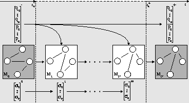Eventually, a sequence of discrete switches terminates in a real mode (system behavior again evolves as a function of time), and the continuous state vector for this new mode has to be derived. This is illustrated in Fig. 3. Mythical modes are depicted in a white background and real modes in a dark background. In real mode a signal value crosses a threshold at time , which causes a discontinuous change to model configuration , represented by the discrete state vector . The power variable values in this new configuration are calculated from the original energy distribution values. If the new values cause another instantaneous mode change, a new mode is reached, where the new power variables values, ( , ), are calculated from the original energy distribution . Further mythical mode changes may occur till a real mode, , is reached. The final step involves mapping the energy distribution, or continuous state variable values, of the departed real mode to the new real mode. This issue is non-trivial, and discussed in detail in a later section. Real time continuous simulation resumes at so system behavior in real time implies mode follows . The formal Mythical Mode Algorithm (MMA) is outlined below.

1. Calculate the energy values ( ) and signal values ( ) for bond graph model using ( , ), values at the previous simulation step as initial values.
2. Use CSPEC to infer a possible new mode given ( ).
3. If one or more controlled junctions switch states then:
   1. Derive the bond graph for this configuration.
   2. Assign causal strokes using the SCAP algorithm[12].
   3. Calculate the signals ( ) for the new mode, , based on the initial values ( ).
   4. Use CSPEC again to infer a possible new mode based on ( ) for the new mode, .
   5. Repeat step 3 till no more mode changes occur.
4. Establish the final mode, , as the new system configuration.
5. Map to the energy distribution for , .

  
Figure 3: State Evolution: Mythical + Real Modes.

A complete simulation system that incorporates continuous simulation and the MMA algorithm been implemented and tested on a number of physical system examples[9].