Practical Information
- Due Date: Tuesday 12 November 2024, before 23:59.
- Team Size: 2 (pair design/programming).
Note that as of the 2017-2018 Academic Year, each International student should team up with "local" (i.e., whose Bachelor degree was obtained at the University of Antwerp). - Submission Information:
- Only one member of each team submits a full solution.
- This must be a compressed archive (ZIP, RAR, TAR.GZ...) that includes your report and all models, images, code and other sources that you have used to create your solution.
- The report must be in PDF and must be accompanied by all images.
- Images that are too large to render on one page of the PDF must still be rendered on the PDF (even though unclear), and the image label should mention the appropriate file included in the submission archive.
- Make sure to mention the names and student IDs of both team members.
- The other team member must submit a single HTML file containing the coordinates of both team members using this template.
- Submission Medium: BlackBoard Ultra. Beware that BlackBoard's clock may differ slightly from yours. If BlackBoard is not reachable due to an (unpredicted) maintenance, you submit your solution via e-mail to the TA. Make sure all group members are in CC!
- Contact / TA: Rakshit Mittal.
Goals
In this assignment, you will learn to create and use Causal-Block Diagrams (CBD) using the pyCBD framework created by our lab. You will continue to use the plant model for the gantry system you built in the Modelica assignment. You will learn:
- about the numerical analysis, accuracy and stability of your models
- orchestration of coupled CBDs
- the use (and orchestration) of the Functional Mockup Interface (FMI), an industrial standard, used for exchange of simulation models between vendors and customers without exposing valuable Intellectual Property (IP)
- the relation of FMI to Modelica
- in order to get a better understanding about how tools like OpenModelica and MatLab Simulink work behind the scenes.
PyCBD
You will use this Python-based CBD framework for all tasks. The zip-file contains a full Python framework to allow CBD modelling in Python. You can install the Python package within your Python virtual/environment by executing the following command from within the src folder:
pip install .
To view the documentation you can execute the docs.bat or docs.sh scripts. The documentation is already provided in the zip-file. You can view it by opening doc/_build/pyCBD.html in a browser. Additionally, the documentation provides a set of examples which may help you in completing this assignment. Especially the "Sine Generator" example.
Note: The internal implementation of pyCBD will be much more complicated compared to the algorithms introduced in the lectures. If something is not clear, or if you have found an issue/bug, or if you have a feature request, please contact the TA.
Please read the documentation of everything you use! If the documentation explicitly states you cannot do something, don't! If you use a function or a class in a way that disregards the "warning", "danger", "attention"... labels, you will not receive any points on that task, even if it produces the correct results.
Once the simulator is installed, it works with any IDE, including Jupyter Notebooks.
For creating plots of simulation traces, Bokeh, MatPlotLib and SeaBorn are supported.
DrawioConvert
DrawioConvert is an additional tool that allows the creation, visualization and code generation of coupled CBDs. The tool may still have small bugs, and its use is optional, however incredibly useful. It uses DrawIO as a front-end. A small tutorial on how to use the tool is provided. Please contact the TA if you experience any problems.
- DrawIO Library
- Download Python Code
- Requires: Jinja2
You should first install DrawIo from this link
Essentially, using this tool, you can define your CBDs in a graphical environment (much like the graphical editor of OMEdit), and then use the DrawioConvert Python code to generate Python code that instantiates a CBD model based on the PyCBD framework. It simplifies the creation of your CBD and you are encouraged to use it.
Functional Mock-up Interface (FMI) and Functional Mock-up Units (FMU)
FMI (Functional Mock-up Interface) is a standard developed to support the model exchange and co-simulation of dynamic models between different tools. FMI allows various simulation tools to share models and simulations in a unified way, which can greatly simplify the process of combining models developed in different software.
FMU (Functional Mock-up Unit) is a model packaged according to the FMI standard. Essentially, an FMU is a zipped file containing a model and all necessary data and scripts to simulate it. It can be imported and simulated across many tools that support FMI.
In short, an FMU is a zipped package of a specifically structured set of files. Because understanding the details of the FMI Standard is not within the scope of this assignment, we have provided you with a template FMU for CBD models that you can fill with your own code. The template file can be uncompressed, and you can browse the internal files. For your convenience, the only files you need to edit are:
sources/defs.h: Header file that uses#defines for human-readable coding.sources/eq0.c: Should contain the equations for the first iteration.sources/eqs.c: Should contain the equations for all other iterations.modelDescription.xml: Contains the simulation setup and the exposed interface of the FMU.
Note: You will not have to manually create or generate these files in this assignment, since that is out of scope. You will only use the CBD2FMU package to generate an FMU from the CBD model. However, it is good to know the contents of these files and have a basic idea about the structure of an FMU, since your co-simulation script will depend on the contents of the FMUs. For the assignment you will be most interested in modelDescription.xml
sources/defs.h
When you start the process of inline integration, you will get M internal variables. These are the outputs and inputs
of each of the blocks, after the CBD is flattened. The variables allow you to easily write the equations. For instance, an
AdderBlock with two inputs will yield three variables: IN1, IN2 and OUT. For the sake
of convenience, we will expose all variables to the user. This allows us to store them as an array (called modelData) in the
CBD struct (see sources/model.c).
To allow user-readability, you should use the sources/defs.h file to predefine some variables as macros.
For the AdderBlock, an example can be:
				#define M 3  /* Number of Internal Variables */
				#define _Adder_IN1 (cbd->modelData[0])
				#define _Adder_IN2 (cbd->modelData[1])
				#define _Adder_OUT (cbd->modelData[2])
Notice that M is required to be set to the total number of variables. Additionally, you can assume they have access to
a variable called cbd, which is a pointer to the current instance of the CBD struct. Furthermore, you may notice that the C-code
has no knowledge of the past (i.e., the modelData array does not contain timing information). This is especially useful to know
when dealing with DelayBlocks. For the macro names, you are encouraged to use (and encode) the individual block names. This way,
you can understand, debug and verify your own generated code.
sources/eq0.c and sources/eqs.c
The normal inline integration will be yielded in these files. You have access to a variable called cbd, which is a pointer
to the current instance of the CBD struct. You should only need its internal modelData array (see above). Additionally,
there is a variable called delta, which is the time since the previous computation. For the first iteration, this will
be set to 0. For the adder, both the sources/eq0.c and sources/eqs.c
will look as follows:
_Adder_OUT = _Adder_IN1 + _Adder_IN2;
modelDescription.xml
This file contains a lot of information about the general simulation setup. Please only change the described tags of this file. The other files are constructed such that they are linked correctly. Note that the description below and the provided FMU are a massive oversimplification of the total FMI 2.0 reference.
<ModelVariables>: Contains theMinternal variables, denoted as unique<ScalarVariable>s.-
<ScalarVariable>: Has 5 attributes:name(the name of the variable, as exposed to the user),valueReference(the index in themodelDataarray that refers to this variable),initial(how the variable is initialized; "exact" implies that it is known, "calculated" otherwise) (this attribute may not be set for inputs!),causality(kind of parameter; "input" implies model input, "output" is model output, "local" otherwise),variability(how the value will change; "constant" forConstantBlocks, "continuous" otherwise).
<Real>tag as a child, which has astartattribute (indicating the starting value of the variable) if the<ScalarVariable>'sinitialequals "exact", or when it is of causality "input" and variability "continuous". <ModelStructure>: Special cases of the variables. It contains an<Outputs>tag, which has a set of<Unknown>children. There is also an<InitialUnknowns>tag, which will be the exact same as the<Outputs>tag (for the purposes of this exercise). Each<Unknown>has an attributeindex, referring to the corresponding (one-based) index w.r.t. the ordering of theScalarVariables. Only the model outputs are<Unknown>s (for the purposes of this exercise).
An example for the adder is given in this file.
Creating an FMU from Modelica
We can very easily create an FMU from a Modelica model directly from OMEdit, with the following steps:- Go to
Tools > Options > FMIand make sure that:Versionis 2.0,Typeis "Model Exchange and Co-Simulation"Platformsis "Native" (if you intend to co-simulate the FMU on the same computer)
-
Right-click on your Modelica class that you want to export as FMU and select
Export > FMU(this might take a few seconds).
The output panel will show where the FMU has been generated, so you can access it. The output consists of:
- A zipped file with the name
package_name.model_name.fmu - A directory named
model_name_with_hashthat provides logs and other metadata regarding the generated FMU.
You will only be interested in the generated fmu and can disregard the directory with metadata.
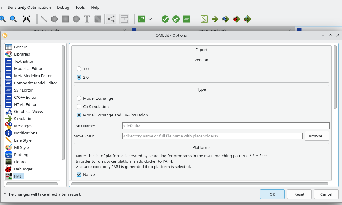
Fig. 1. Settings to ensure for Export of Modelica model to FMU.
Creating an FMU from PyCBD Model
You will use inline integration to create your own FMU that will be used in cosimulation. Because understanding the generation of FMUs is out of scope for this assignment, we have provided you this Python package created by our lab member Randy Paredis as part of his PhD thesis. This zip-file contains a Python project to generate FMUs from CBD models.
You will find the main function in src/generator.py. Look at the Bouncing Ball example, you can either manually copy the CBD module into the main method, or use the code to load the model automatically from another file.
The executable C-code is created by doing a topological sort for all blocks and iteratively turning each block into their corresponding equation(s). This also takes the internal connections into account. This method is called "Inline Integration". This paper (see especially table 2) somewhat explains the process for inline integration of CBDs (mainly focusing on LaTeX generation). Notice that the dependency graph at iteration 0 will differ from the graph at all other times, so the inline integration needs to happen twice. For the purposes of this assignment, we will ignore how algebraic loops can/should be solved.
Also have a look at this report (of a project for the Model Driven Engineering course) explaining the generation of FMUs from CBDs and the advantages of doing so (including lower computation time)
Note: The FMU generated with CBD2FMU only contains model.c which contains code from both eq0.c and eqs.c that are described above.
Assignment Overview
Integration Methods
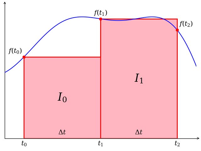
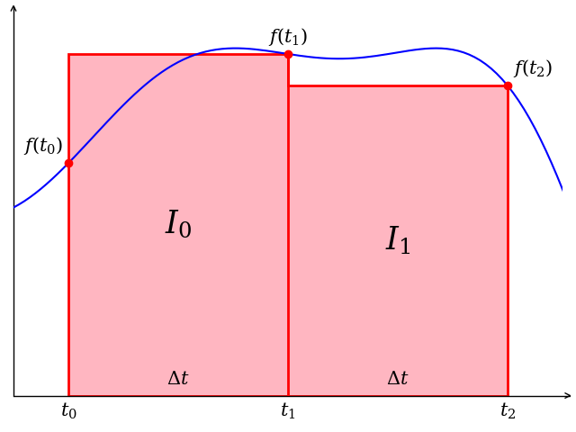
Computing the integral of a function is a common practice in simulation systems. It can be used for specifying time-dependent simulations, constructing (PID) controllers and even identifying accumulative errors. Any complex Cyber-Physical process that happens over a certain period of time makes use of integrators, however their computation is always a numerical approximation. This task will take a look at multiple integration methods and their accuracy. Table 1 shows the four integration methods we will concern ourselves with for this assignment (note: there exist many, many more).
 |
 |
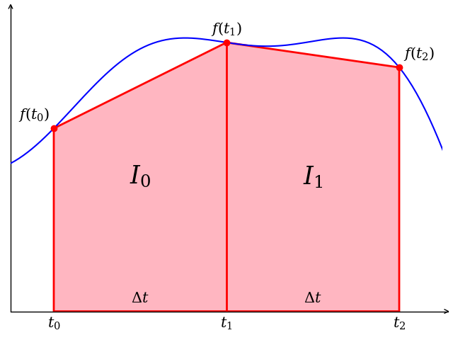 |
| Backwards Euler Method | Forwards Euler Method | Trapezoid Rule |
| $$I_0 = f(t_0)\cdot \Delta t$$$$I_1 = f(t_1)\cdot \Delta t$$$$I = I_0 + I_1$$ | $$I_0 = f(t_1)\cdot \Delta t$$$$I_1 = f(t_2)\cdot \Delta t$$$$I = I_0 + I_1$$ | $$I_0 = \dfrac{f(t_0) + f(t_1)}{2}\cdot \Delta t$$ $$I_1 = \dfrac{f(t_1) + f(t_2)}{2}\cdot \Delta t$$ $$I = I_0 + I_1$$ |
| computed over 1 iteration | computed over 1 iteration | computed over 1 iteration |
Tasks
Your job is to compare the given integration methods.
-
For each of the given integrators, implement a coupled CBD block.
- The backwards Euler method is already implemented in the CBD framework in CBD.lib.std.IntegratorBlock. However, you have to create one on your own.
Note: An excellent self-test is to check if the implementation in the CBD framework corresponds to your implementation, if you are using DrawioConvert. - Each integrator block should have an initial condition input (which is called IC), that outputs this value at the first iteration.
- Include images that show the created CBDs visually. Make sure they are clearly readable.
- The backwards Euler method is already implemented in the CBD framework in CBD.lib.std.IntegratorBlock. However, you have to create one on your own.
- For the function $g(t) = \dfrac{t + 2}{(t + 3)^2}$, it is known that the integral over the range $[0, 100]$ is: $$\int_3^{103} (\dfrac{1}{u} - \dfrac{1}{u^2}) du = \left[\dfrac{1}{u}+\ln(|u|)\right]_3^{103} = 3.212492104$$ Implement $g(t)$ as a coupled CBD block. It will have a single input from the clock, and a single output as the value of the function at time t.
- Create another coupled CBD block for each integrator, with the function $g(t)$ such that the integral of $g(t)$ is the output. Compute and compare the integral of $g(t)$ for $\Delta t = 0.1$, $\Delta t = 0.01$ and $\Delta t = 0.001$, using the three different integrators.
Make sure to also compare against the analytical solution! Which one(s) is/are the most accurate?
Hint: this will result in 10 different values (= 3 different $\Delta t$, using 3 integrators + 1 analytical solution) to compare.
Co-simulation
Note: This task assumes you know the C programming language. A simple tutorial can be found on the
W3 Schools Website While this is not a strict requirement, you need it to understand the generated C-code from your PyCBD model.
Note: Additionally, it is assumed you have fully completed the previous (Modelica) assignment. Do not make changes to your Modelica assignment until you have submitted it!
Even though you have a CBD simulator, its execution in Python is slow. Sometimes, models need to be executed on minimal hardware that may not have the computational power (and storage) to run the model. This is in particular true if we want real-time execution of our simulation. To obtain a fast simulator, the (Open)Modelica first expands object-oriented constructs and then flattens a model, subsequently assigns causality and sorts equations and finally generates C code. Finally, this C code representing the causality assigned and sorted equations is compiled and linked with compiled numerical solver code (from a library).
If we have a model containing multiple sub-models, these sub-models may be compiled independently. Sub-models may be Modelica models or CBD models. The different sub-model simulators now need to be "orchestrated" as explained in class. This is called co-simulation. The industrial standard for co-simulation is the Functional Mock-up Interface (FMI). A single instance (sub-)model is called a Functional Mock-up Unit (FMU). For this assignment, we will use the FMI standard version 2.0 as it is simpler than the current 3.0 version.
In the previous assignment, you modeled the gantry system and its PID controller in a single Modelica file. However, in practice, the controller and plant may be designed by completely different teams with their own models and formalisms. In our assignment:
- The team designing the actual mechanical components of the plant model is using Modelica.
- The team designing the controller is using the CBD formalism with the PyCBD package. In reality, they would like to have a controller algorithm that can be embedded on a real system. Hence, C-code needs to be generated from the PyCBD classes, which can then be compiled into an FMU.
The teams may be part of the same organization, or they may have hired a consultant in order to design the controller for their plant. If you have partnered with another entity, it is vital for both of you to protect your Intellectual property in order to maintain competitiveness, hence you have agreed to share models using the FMI 2.0 standard.
Tasks
In this part of the assignment, you will impersonate both these teams:- You will first create an FMU from the Modelica model of the plant system (only!) and not the entire PID control loop.
- Then you will create a PID controller using the PyCBD formalism
- You will then generate C-code for the PID-controller CBD
- Finally, you will compile and co-simulate both the FMUs, together.
The co-simulation architecture will look like the following (notice the similarity to the PID control loop from the Modelica assignment. We are essentially doing the same thing, but this time, with the power of co-simulation.):
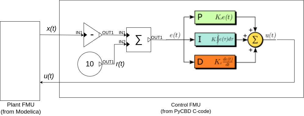
Fig. 2. Co-simulation architecture for this task.
Notice that part of the Control FMU is expressed in PyCBD Drawio concrete syntax. However, in the task, you will fully express the control FMU in PyCBD (you may or may not use Drawio), and then generate C-code from it.
Sub-task 1: Plant FMU from Modelica
-
In Modelica, export ONLY(!!) the plant block (which contains only the gantry system model) to FMU. Follow the steps described in this section. Ensure that your model does not contain any values for input signals. There should be one input and two outputs from this block. The input is the control signal, and the output are the position and angular displacement of the gantry system.
Note: You may not have created the second output from the Modelica model for the angular displacement. You should add it as another real output and equate it to the value of the angular displacement, before exporting the FMU. - Rename the fmu to "Plant.fmu"
Sub-task 2: PID Controller in PyCBD
- Create a PID controller using PyCBD. You may use DrawIo and generate Python code, or directly write Python code, as you prefer.
-
Use
ConstantBlocks for $K_p$, $K_i$ and $K_d$, which should (by default) have your solution from the last assignment (add $K_i = 1$).
Note that this will hardcode these values in your solution. We will do this for the sake of simplicity. -
The controller's input (called
IN) will be given the linear displacement value $x(t)$, as defined in the previous assignment. - The controller internally defines a constant set-point of 10, mimicking the same scenario, as used for the PID control parameter tuning in the Modelica assignment.
-
The controller's output
(called
OUT) will yield $u(t)$. - Include a graphical representation of this CBD model in your report.
Sub-task 3: Controller FMU from Controller CBD
Use this Python package to generate the FMU for the controller, from the PyCBD model.
Report the contents of description.xml, sources/model.c and correlate it with the description of FMUs
Sub-task 4: Compile Controller C-Code and Co-simulate
- Install FMPy and download the compile_and_run.py orchestration script.
-
Read and understand the orchestration script. We will use this for cosimulation. It is currently incorrect for your FMUs; you will have to modify it. Basically this file describes a configuration for an FMU (called Container.fmu) that couples the two constituent FMUs (Plant.fmu and Controller.fmu). Then the FMU is compiled and simulated, and the resulting traces are available in the
resultsvariable. Take a note of the definitions of variables, components, and connections in the configuration of Container.fmu:- The components specify the constituent FMUs, (in our case, the controller and the plant.)
- The connections specify the causal connections between these components. Refer to Fig. 2, in which it is clearly shown that there are 2 connections: the plant provides the linear displacement $x(t)$ to the controller, and the controller provides the control signal $u(t)$ to the plant.
- The variables specify which variables should be produced from the simulation of the co-simulated FMUs. In our case, this would be both, the linear displacement, and the angular displacement associated with the gantry. So you should make sure that both these variables are defined.
-
Modify the script to ensure the above requirements are met. Also make sure to set an appropriate step-size and stop-time. The modifications depend on:
- The names of inputs and outputs in your Modelica block.
- The name you used to instantiate the controller model, when you generated the FMU from PyCBD, using CBD2FMU.
- The names of input and output blocks in your controller's PyCBD model.
- Run the orchestration script and create a plot from the traces of linear and angular displacement of the Gantry system.
- The resulting plot should be the same as the ones obtained from Modelica. Include both in this report and show/prove they are the same.
Please contact the TA if you have any questions, or get stuck whilst working on this assignment. The goal of this task is to help you realize how CBD models can be converted into executable code, how it is done in industry. You are not required to understand all FMI details, or to get stuck in debugging C-code.
Practical Issues
- All parts of this assignment use Python 3.6+. Do not use features from Python 2.7 (discontinued as of January 1, 2020).
- The files for DrawioConvert can be found here:
- FMU Co-Simulation Orchestration Script: http://msdl.uantwerpen.be/people/hv/teaching/MoSIS/assignments/CBD/compile_and_run.py
- Useful documentation:
- The CBD Simulator's documentation
- CBDs: http://msdl.uantwerpen.be/people/claudio/pub/Gomes2016a.pdf
- C programming: https://www.w3schools.com/c/index.php
- FMPy: https://pypi.org/project/FMPy/