Our transient-based diagnosis scheme has been successfully applied to a number of different hydraulic systems (see http://air.vuse.vanderbilt.edu:8080/ for a working version of the system) [7]. To investigate scalability of the measurement selection algorithm we applied it to the model of the secondary cooling loop of a fast breeder reactor. The need for a qualitative approach to fault detection and isolation in this system is motivated by its high-order (six), nonlinearity, and the non availability of precise and real-time numerical simulation models. The precision of flow sensors is limited by signal noise, and achieving hardware redundancy by installing flow sensors is expensive.
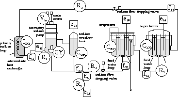
Heat from the reactor core is transported to
the turbine by a primary and secondary cooling system.
Liquid sodium is pumped through an
intermediate heat exchanger to transport heat from the primary cooling
loop to the feed water loop by means of a superheater and
evaporator vessel (Fig. 7).
Pump losses are modeled by ![]() .
The coil in the intermediate heat exchanger that accounts for
flow momentum build-up is represented by a fluid
inertia,
.
The coil in the intermediate heat exchanger that accounts for
flow momentum build-up is represented by a fluid
inertia, ![]() .
The two sodium vessels are capacitances,
.
The two sodium vessels are capacitances,
![]() and
and ![]() .
An overflow column,
.
An overflow column, ![]() , maintains
a desired sodium level in the main motor.
All connecting pipes are modeled as resistances.
, maintains
a desired sodium level in the main motor.
All connecting pipes are modeled as resistances.

Figure 7: Secondary sodium cooling loop.
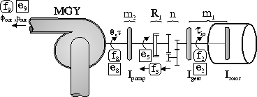
The main motor driver (Fig. 8) is a
synchronous, ![]() motor,
and as an assumption,
its electrical field is considered to be
present as soon as it is turned on.
Therefore, dynamic electrical effects are not modeled,
and the electrical part of the motor system can be represented as a source
of mechanical energy with a given torque/angular velocity characteristic.
The inertia of the rotor and the mass of transmission gear
is modeled by
motor,
and as an assumption,
its electrical field is considered to be
present as soon as it is turned on.
Therefore, dynamic electrical effects are not modeled,
and the electrical part of the motor system can be represented as a source
of mechanical energy with a given torque/angular velocity characteristic.
The inertia of the rotor and the mass of transmission gear
is modeled by ![]() , and the transmission
ratio between motor and pump by n. Pump losses in the
fluid connection between the motor and pump are modeled by a dissipation
element,
, and the transmission
ratio between motor and pump by n. Pump losses in the
fluid connection between the motor and pump are modeled by a dissipation
element,
![]() , and the pump inertia is represented as
, and the pump inertia is represented as ![]() .
The model of a centrifugal pump can be derived using conservation of power
and momentum [6].
The pump is represented by
.
The model of a centrifugal pump can be derived using conservation of power
and momentum [6].
The pump is represented by
![]() which
describes a modulated gyrator with modulus
which
describes a modulated gyrator with modulus ![]() .
If the pump veins are not curved, b = 0.
.
If the pump veins are not curved, b = 0.

Figure 8: Pump driven by an ac motor.
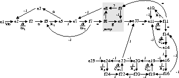
The derivation of the causal relations of the sodium pump
are based on a
modulation factor g between input angular velocity, ![]() , and
output flow rate,
, and
output flow rate, ![]() ,
, ![]() . This factor is directly
proportional to
. This factor is directly
proportional to ![]() and inversely proportional to
and inversely proportional to ![]() ,
,
![]() . The dependency of g on
. The dependency of g on ![]() and
and ![]() can
be explicitly modeled by edges between these variables and the
affected variables. In case of the dynamic behavior, the affected variables
are input torque,
can
be explicitly modeled by edges between these variables and the
affected variables. In case of the dynamic behavior, the affected variables
are input torque, ![]() , and output pressure,
, and output pressure, ![]() ,
and the corresponding edges
are added to the causal graph (Fig. 9).
,
and the corresponding edges
are added to the causal graph (Fig. 9).

Figure 9: Temporal causal graph.
The dependency on system variables of the modulation factor
results in nonlinear, quadratic, behavior
![]() , and, therefore, the relation on the
edge between
, and, therefore, the relation on the
edge between ![]() and
and ![]() is unknown, in general.
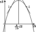
A sensitivity analysis of this
relation, shown in Fig. 10, reveals that depending
on the values of
is unknown, in general.
A sensitivity analysis of this
relation, shown in Fig. 10, reveals that depending
on the values of ![]() and
and ![]() , the sensitivity of
, the sensitivity of ![]() to
to ![]() is positive or negative. Given the nominal values of the steady
state operation of the system, which is parameter dependent,
the weight of
is positive or negative. Given the nominal values of the steady
state operation of the system, which is parameter dependent,
the weight of ![]() can be determined as a positive
(1) or negative (-1) influence. However, once a deviation
occurs,
can be determined as a positive
(1) or negative (-1) influence. However, once a deviation
occurs, ![]() and
and ![]() may differ from their nominal values
and a different operating point may be reached. Since these
new values are caused by failure, and, therefore, unknown,
the influence may reverse and is unknown as well.
Because this can only occur if
may differ from their nominal values
and a different operating point may be reached. Since these
new values are caused by failure, and, therefore, unknown,
the influence may reverse and is unknown as well.
Because this can only occur if ![]() is predicted to be high based on the proportional influence (-1 or 1),
only a predicted decrease in
is predicted to be high based on the proportional influence (-1 or 1),
only a predicted decrease in ![]() is unambiguous, and, therefore,
propagated. A predicted increase in
is unambiguous, and, therefore,
propagated. A predicted increase in ![]() is propagated as
unknown.
is propagated as
unknown.

Figure 10: Detailed sensitivity analysis of
![]() .
.