Measurement selection is critical to
designing an economically viable and effective monitoring and fault
isolation system.
The measurement selection algorithm (Algorithm 1) works
off-line. Given the set of measurements that can be made on the system
and the set of possible faults, i.e., parameter deviations, the
algorithm derives subsets of measurements that can uniquely isolate
all individual faults. For all possible
parameter deviations, j, (above and below normal) signatures, s[i,j],
for all observations, i, are generated.
For every observation i, the signatures of pairs of faults (j,k) are
compared and entries made into a discrimination matrix ![]() . If
the signatures of faults j and k differ,
. If
the signatures of faults j and k differ, ![]() is set to
0, otherwise it is set to 1. The discriminatory ability of two
measurements, say p and q, is defined as
is set to
0, otherwise it is set to 1. The discriminatory ability of two
measurements, say p and q, is defined as
(1) ![]()
This procedure can be applied to compute the discrimination matrix for a subset of measurements. When the combined discrimination matrix equals the identity matrix, all faults are distinguishable.


The measurement selection algorithm
was implemented in Visual Basic Pro 3.0.
Measurement selection of the secondary liquid sodium
cooling system described
in the next section for ![]() order signatures
is performed in two minutes on a 200MHz Pentium Pro with 32MB of RAM.
order signatures
is performed in two minutes on a 200MHz Pentium Pro with 32MB of RAM.
To illustrate this algorithm, consider the bi-tank system in Fig. 1. Possible measurement points are selected to be the left and right outflow, the flow from the left to the right tank, and the pressure in both tanks. The component parameters of the system are the left and right tank capacities and the flow resistances. First, magnitude changes in the observed variables are determined for positive deviations of all parameters, which yields:
Similarly, slopes of all observable signals are determined for all positive parameter deviations:
The effects of negative parameter deviations are computed analogously.
In this system, these influences are the opposite of positive parameter
deviations.
An exhaustive search is now applied to
identify which set of minimal measurements produces unique feature
characteristics for all parameter deviations. To this end, 0
value slopes are not used because they may be ambiguous [6].
The discrimination matrix for observation ![]() is compiled as
is compiled as
(4) 
This indicates that faults in
![]() cannot be distinguished by observation
cannot be distinguished by observation
![]() alone.
If
alone.
If ![]() is added as an observation, the discrimination matrix of
is added as an observation, the discrimination matrix of
![]() becomes
becomes
(5) 
This implies that ![]() cannot be distinguished with
cannot be distinguished with
![]() as observations.
Inspecting the matrices in (2) and (3)
one learns that
for these observations parameter deviations in
as observations.
Inspecting the matrices in (2) and (3)
one learns that
for these observations parameter deviations in ![]() and
and ![]() have the same magnitude deviations.
Though the slopes
differ between normal (bold faced)
and a non-normal value, typically this
cannot be used to refute either of the two faults.
This is an interesting result because
have the same magnitude deviations.
Though the slopes
differ between normal (bold faced)
and a non-normal value, typically this
cannot be used to refute either of the two faults.
This is an interesting result because
![]() constitutes the system state in
a systems theory sense [4].
So, simply observing the state of a system may not
be the most effective for fault isolation.
If only
constitutes the system state in
a systems theory sense [4].
So, simply observing the state of a system may not
be the most effective for fault isolation.
If only ![]() order signatures are used,
and discontinuities can be detected,
the system is completely diagnosable for the observation sets
order signatures are used,
and discontinuities can be detected,
the system is completely diagnosable for the observation sets
![]() ,
, ![]() , and
, and ![]() .
Alternatively, if
.
Alternatively, if ![]() order signatures are used, the system
is completely diagnosable for
order signatures are used, the system
is completely diagnosable for
![]() ,
, ![]() ,
, ![]() ,
, ![]() ,
and
,
and ![]() .
This is due to progressive monitoring which replaces normal values
of predicted
.
This is due to progressive monitoring which replaces normal values
of predicted ![]() order derivatives with non-normal predicted
order derivatives with non-normal predicted
![]() order derivatives if available.
So
order derivatives if available.
So ![]() order signatures require
one less observation, but require more measurement points in time
for fault isolation since
order signatures require
one less observation, but require more measurement points in time
for fault isolation since ![]() order effects have to propagate in the
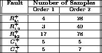
system (see Table 1).
During this time, abnormal system values may cause cascading faults,
leading to fault masking.
order effects have to propagate in the
system (see Table 1).
During this time, abnormal system values may cause cascading faults,
leading to fault masking.

Table 1: Delay times in fault isolation when failing with
a factor 5, ![]() , margin = 5%.
, margin = 5%.