The diagnosis methodology based on a qualitative reasoning framework incorporates three primary tasks: (i) initial fault implications from observed deviations, (ii) prediction of observed behaviors for hypothesized faults, and (iii) monitoring to refine the hypothesized fault set [6, 9, 7].
![]()
A first step in fault isolation is to detect when observations deviate from their nominal values. Nominal values are typically available from design documents, operators manuals, or simulation models, and depending on the nature and quality of the sensor, a measurement is reported to be deviant (above or below normal) if its percentage deviation is greater than 2-5% of the nominal value. Typically, deviations are recorded in terms of their magnitude and slope changes in dynamic systems [1, 6].
As discussed earlier, continued monitoring of the actual
magnitude deviations and slopes of observations is then used to prune the
hypothesis space. To this end, future behavior of the system for each
of these parameter deviations is predicted in qualitative
terms of their time-derivative changes. Predicted effects of
deviations can often be of ![]() or higher order, depending on
the number of energy storage elements in the system [6].
Typically, measuring higher order derivatives is unrealistic, especially
in noisy environments [1]. In previous work, we have
discussed an innovative scheme, called progressive monitoring,
where higher order derivatives are
propagated down to slope and magnitude changes for observations
to predict their future behaviors.
or higher order, depending on
the number of energy storage elements in the system [6].
Typically, measuring higher order derivatives is unrealistic, especially
in noisy environments [1]. In previous work, we have
discussed an innovative scheme, called progressive monitoring,
where higher order derivatives are
propagated down to slope and magnitude changes for observations
to predict their future behaviors.
Our system model for diagnosis analysis is a temporal causal graph,
derived from a bond graph model [9, 7].
This graph captures
relations between system variables, which are typically effort and
flow variables. Relations capture instantaneous magnitude relations
expressed in terms of component parameter values, and temporal
effects (dt relations) introduced by energy storage elements
which eliminates
problems with feedback loops in physical systems.
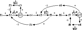
As an example, consider the bi-tank system in Fig. 1
and its temporal causal graph
in Fig. 2. The inflow ![]() affects the total inflow,
affects the total inflow, ![]() ,
into tank 1 with capacity
,
into tank 1 with capacity
![]() in direct proportionality. The outflow on the left of
in direct proportionality. The outflow on the left of ![]() equals
the flow through
equals
the flow through ![]() ,
, ![]() , which affects
, which affects ![]() in inverse
proportionality.
The outflow,
in inverse
proportionality.
The outflow, ![]() , on the right of
, on the right of ![]() , equals the flow,
, equals the flow, ![]() , through
, through
![]() inversely related to
inversely related to ![]() . This is indicated by a -1 sign on
the edge. The net flow
. This is indicated by a -1 sign on
the edge. The net flow ![]() into
into ![]() is related to the amount of stored liquid in the tank based
on an integrating relation, which appears as the relation between
the pressure
is related to the amount of stored liquid in the tank based
on an integrating relation, which appears as the relation between
the pressure ![]() and flow
and flow ![]() as a time-derivative
effect,
as a time-derivative
effect, ![]() .
.

Figure 2: Temporal causal graph of the bi-tank.
Details of the algorithms that are outlined next appear in [9].