This module compares reported signatures and
actual observations as they change dynamically
after faults have occurred.
Transients generated by failures are dynamic, therefore,
the signatures of
the observed variables change over time. For example, at time
step 1 in Fig. 5 a variable has a magnitude reported normal
and a ![]() derivative
which is above normal. Over time the variable value will
go above normal, and at time stamps marked 2 and
3 a lower order effect is replaced by manifested higher order
effects.
Incorporating effects of
higher order derivatives in the comparison process is referred to as
progressive monitoring.
derivative
which is above normal. Over time the variable value will
go above normal, and at time stamps marked 2 and
3 a lower order effect is replaced by manifested higher order
effects.
Incorporating effects of
higher order derivatives in the comparison process is referred to as
progressive monitoring.

Figure 5: Dynamics of higher order derivatives.
Progressive monitoring is activated
when there is a discrepancy between a predicted value and
a monitored value that deviates
(this applies to ![]() and higher order
derivatives). At every time point, it is
checked whether the next higher derivative could make
the prediction consistent with the observation. If this
next higher derivative value is normal the next following
higher derivative value is considered, until there is either a conflict in
prediction and observation, a confirmation, or an unknown
value is found. Note that this implies that normal values are not
explicitly used to refute fault hypotheses. Also note that this means
that step 3 in Fig. 5 is not executed. Rather, at that
point in time, transient verification is suspended in favor of
steady state detection [6].
If discontinuities can
be detected, progressive monitoring does not affect the
and higher order
derivatives). At every time point, it is
checked whether the next higher derivative could make
the prediction consistent with the observation. If this
next higher derivative value is normal the next following
higher derivative value is considered, until there is either a conflict in
prediction and observation, a confirmation, or an unknown
value is found. Note that this implies that normal values are not
explicitly used to refute fault hypotheses. Also note that this means
that step 3 in Fig. 5 is not executed. Rather, at that
point in time, transient verification is suspended in favor of
steady state detection [6].
If discontinuities can
be detected, progressive monitoring does not affect the
![]() order derivative, and, therefore, when it is predicted to be
normal, it can still refute faults [6].
order derivative, and, therefore, when it is predicted to be
normal, it can still refute faults [6].
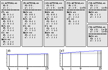
Consider a sudden increase in outflow resistance ![]() .
Fig. 6 shows the results of progressive
monitoring, where at times
the signatures of the observed variables are modified because of
higher-order effects.
For example, the signature of
.
Fig. 6 shows the results of progressive
monitoring, where at times
the signatures of the observed variables are modified because of
higher-order effects.
For example, the signature of ![]() for
for ![]() changes from 0,0,1 in step 1 to 1,1,1 in step 9. The
changes from 0,0,1 in step 1 to 1,1,1 in step 9. The ![]() order derivative, which is positive, is assumed to have affected
the magnitude to make the candidate
consistent with the observation 1,1,. in step 9.
Discontinuity
detection was not employed.
When discontinuity detection was
used, the same end result was obtained in three steps [7].
Note that only
order derivative, which is positive, is assumed to have affected
the magnitude to make the candidate
consistent with the observation 1,1,. in step 9.
Discontinuity
detection was not employed.
When discontinuity detection was
used, the same end result was obtained in three steps [7].
Note that only ![]() and
and ![]() order derivatives of the
observations are available, as opposed to the predictions which include
order derivatives of the
observations are available, as opposed to the predictions which include
![]() order derivatives as well.
order derivatives as well.

Figure 6: Progressive monitoring for fault ![]() .
.